
Estimating the Parameters of Covid-19 Cases in South Africa
 , Poonam Garg2*, Ritu Arora3 and Dhiraj Kumar Singh4
 1Department of Mathematics, Shivaji College (University of Delhi), Raja Garden, New Delhi 110027, India.
2Department of Mathematics, Deen Dayal Upadhyaya College (University of Delhi), Azad Hind Fauj Marg, Dwarka, Delhi 110078, India.
3Department of Mathematics, Janki Devi Memorial College (University of Delhi), Sir Ganga Ram Hospital Marg, New Delhi 110060, India.
4Department of Mathematics, Zakir Husain Delhi College (University of Delhi), Jawaharlal Nehru Marg, Delhi 110002, India.
Corresponding Author E-mail: pgarg@ddu.du.ac.in
DOI : http://dx.doi.org/10.13005/bbra/2974
Download this article as:
![]()
In this paper we employ SIR model to study the Covid-19 data of South Africa for a chosen period. This model is solved using three numerical methods, namely, Differential Transform Method (DTM), Multistage Differential Transform Method (MsDTM), Repeated Multistage Differential Transform Method (RMsDTM) to obtain approximations of the number of susceptible, active infected and recovered in South Africa for 60 days starting from June 1, 2021. The proximity of the solution of the RMsDTM to the actual data in comparison to solutions using the other two methods was observed. MsDTM is an improvement over DTM as it uses updated values of the variables as new initial conditions at each iteration of the method. RMsDTM, in which the values of parameters are also changed at suitable intervals of time, besides using updated values of variables is a further improvement over both these methods.
KEYWORDS:Approximation,; Covid-19; Differential Transform Method (DTM); Multistage Differential Transform Method (MsDTM); Pandemic; Repeated Multistage Differential Transform Method (RMsDTM); South Africa; SIR Model
Introduction
Time and again, many pandemics have wrecked havoc on mankind. Spanish flu, almost a century ago; H1N1 Swine flu pandemic, a decade back; and from recent past – the Ebola and Zika virus pandemics have affected mankind adversely. Coronavirus disease is a highly contagious disease caused by SARS-CoV-2 1. Post its probable initiation in Wuhan, China, in December 2019, it spread rapidly across the globe, turning into one of the worst pandemics that human civilisation has ever seen. The Coronavirus was a novel virus, causing mild to moderate respiratory illness in most of the affected people. However, in some cases, the virus also led to serious diseases, sometimes even leading to death. There has been extensive research to understand the behaviour of this virus, in order to contain its spread and cure the infected. Many lives have been lost and a huge economic crisis has engulfed several countries due to the restrictions in travel and trade. Epidemics are region-specific and each country is equipped to handle epidemics affecting their territory. However, a pandemic spreads to several countries and sometimes affects the whole world. The response of each country to the same disease varies and is dependent on its socio-economic structure. A developed country’s preparedness may also not be sufficient to handle such pandemics due to social behaviour, as could be seen in the first wave of Covid-19 in the United States, United Kingdom and Italy. On the other hand, many developing countries like Africa, have been able to contain its spread.
Several Mathematical models like SIS, SIR, SIRD, SEIRD etc., have been developed and employed to study the behaviour of epidemics and make predictions 2. Many such models have been utilized to study this new virus as well 3 in order to predict the number of infected, so that the medical systems are well equipped to handle the predicted number of cases at a given time.
SIR model is a classic compartmental model that was introduced in early 20th century 4. The three compartments of this model, as shown in Figure 1, consist of the susceptible, 𝑠(𝑡), representative of that component of the population who have not been infected and are probable infectives; the infected, 𝑖(𝑡), standing for individuals who have been infected and are capable of spreading the infection and the recovered/removed, r(𝑡), which include those who have recovered from the infection and developed immunity, as well as the deceased. In this model, the members of 𝑟 compartment cannot re-enter the 𝑠 compartment. The total population, 𝑛, is considered to be fixed i.e. 𝑛 = 𝑠 + 𝑖 + 𝑟. The rate of transmission at which susceptible get infected is 𝛽 and the rate at which infected get recovered is 𝛾.
 |
Figure 1: Sir Compartmental Model |
The following system of differential equations is formed for the SIR model5

In this paper we employ SIR model to study the Covid-19 data of South Africa for a period of 60 days 6. In South Africa, the first Covid-19 patient was confirmed on 5th March 2020 7. The person who tested positive for the virus being a thirty-eight-year old man who had returned from a trip to northern Italy 8. Since then, the country has seen several peaks in the number of daily infections, caused due to many variants. In fact, in August most mutated Covid variant C.1.2 was also detected in South Africa. The South African government has continuously been monitoring the pandemic situation and imposing or relaxing restrictions like lockdown, air-travel ban etc. from time to time 9. In this paper, we have undertaken the study of Covid-19 data for a portion of the period of the third wave, starting from 1st June, 2021 to 30th July, 2021.
The paper is organised as follows: The Differential Transformation Method (DTM) is explained in Section 2. In this section, we also initiate a case study of the Covid-19 pandemic scenario for the above stated period using Differential Transform Method on SIR model. The case study is extended in Section 3 using the Multistage Differential Transform Method (MsDTM). We introduce Repeated Multistage Differential Transform Method (RMsDTM) in Section 4 and obtain the estimations of the undertaken case study using this method. A comparison of the outcomes of the three methods is attempted in Section 5. We have given the conclusion of the paper in Section 6.
Differential Transform Method (DTM)
Methodology. The Differential Transform Method dates back to 1986 when Zhou in his paper 10 on linear and nonlinear initial value problems in electric circuits introduced and applied the method to obtain an approximation of the solution. Due to better approximations of the solution in comparison to other methods for solving such systems, DTM has since been used extensively to study initial value problems of systems of linear and nonlinear ordinary differential equations and also systems of partial differential equations 11, 12, 13
Let 𝑓 be a function defined on some open interval containing a point 𝑐. If 𝑓 possesses derivatives of all orders at 𝑐, then the series

is called the Taylor series for 𝑓 about 𝑐. In particular, Taylor series for 𝑓 about 𝑐 = 0 is given by

The 𝑘-th differential transform of 𝑓(𝑥), denoted by 𝐹, is defined as

The function 𝑓 is obtained as an inverse differential transform as follows

Some algebraic and analytical properties of the transform function are listed in Table 1
 |
Table 1 |
In Differential Transform Method, the function 𝑓 is approximated by finite degree polynomial of arbitrary degree 𝐾, i.e.

The remainder terms of the series in equation (1) represent the error in the above approximation and is negligibly small.
DTM for SIR model for Covid-19 in South Africa
In this section we use DTM to solve the SIR model to find susceptible, active infected and recovered of Covid-19 cases in South Africa, for a chosen time period. If 𝑠(𝑡), 𝑖(𝑡) and 𝑟(𝑡) represent the number of susceptibles, active infections and recovered at time 𝑡 and 𝑆, 𝐼 and 𝑅 are their respective differential transform then the transformed system for SIR model is 14

We consider a period of 60 days, starting from 1st June, 2021. The initial conditions on 𝑠, 𝑖 and 𝑟, as obtained from actual data, and the parameters used 15 are as follows

Using the inverse differential transform, the approximation of the polynomials for 𝑠, 𝑖 and 𝑟 upto degree 2 were found to be

The graphs in Figure 2 show the infectives and recovered found using the above solution for the period of 60 days, along with the actual infectives and recovered of that period.
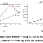 |
Figure 2: (a) Estimated infectives using DTM and actual infectives (b) Estimated recovered using DTM and actual recovered |
In DTM, the number of infected and recovered were obtained using the polynomials given in 2. These are quadratic polynomials, each with positive leading coefficient. So, these are increasing functions for 𝑥 ≥ 0. This is the reason for the number of infected and recovered obtained using this method to be increasing. Whereas in actual data, the numbers are not showing such pattern.
Multistage Differential Transform Method (MsDTM)
Methodology
Multistage Differential Transform Method (MsDTM) 16, 17 is an extension of DTM. In this method, the initial value of the function is dynamically updated at equal intervals of time (Tools of Mathematica 18 have been used for these calculations.). This leads to a better approximation of the We assume that the interval [0, 𝑇] is partitioned into 𝑝 𝑠ub-intervals [𝑡i–1, 𝑡i], 𝑖 = 1, … , 𝑝, where 𝑡0 = 0 and 𝑡p = 𝑇. The sub-intervals are of equal length ℎ, where, ℎ = 𝑇/𝑝. DTM is applied to the first sub-interval, i.e. [0, 𝑡1] with the given initial conditions, to obtain the approximate value of the function at time 𝑡1. This value is now taken as the initial condition for the second interval, [𝑡1, 𝑡2] and DTM is applied. However, here and in subsequent intervals, the Taylor series for 𝑓 about the point 𝑡i–1 is considered for obtaining the solution. In the i-th sub- interval, the solution is given by

So, the function is approximated in [0, 𝑇] as

where
![]()
MsDTM for SIR model for Covid-19 in South Africa
The case study initiated in Section is now attempted using MsDTM. The period of 60 days is sub-divided into 30 periods, each of length 2 days. So, 𝑝 = 30 and ℎ = 2. Using the polynomials obtained at each step and resetting the initial conditions as explained, the values of 𝑠, 𝑖 and 𝑟 were obtained for the period of 60 days (values for 2 days at each step).
The graphs in Figure 3 show the number of infectives and recovered obtained using MsDTM in comparison to the actual data.
 |
Figure 3: (a) Estimated infectives using MsDTM and actual infectives (b) Estimated recovered using MsDTM and actual recovered |
In MsDTM at each step a different quadratic polynomial is obtained for the number of infected and recovered. However, as per the method, the polynomials obtained in successive iterations agree at the last values of these parameters obtained in the previous and the values taken as initial conditions for the succeeding iteration. So, the graph is a joined graph of different quadratic polynomials, with leading coefficient of each being positive. This justifies the increasing graphs, as seen in Figure 3.
Repeated Multistage Differential Transform Method (RMsDTM)
Methodology
Multistage Differential Transform Method has an advantage over DTM in terms of dynamic updating of function’s values during the process at regular intervals of time. There is however no change in the parameters of the system throughout the process. However, in practical situations the parameters also change with time, specially if the time period is long. For instance, the parameters and in SIR model represent the rate of transmission and rate of recovery respectively. These rates fluctuate over a period of time depending on various factors like lockdown, climate, state of vaccination, medical facilities etc. Keeping this in view, we propose a method of repeatedly applying MsDTM with changed parameters at every interval, besides using the updated values of the function as the new initial conditions.
In Repeated Multistage Differential Transform Method (RMsDTM) 19, the interval is divided into suitable sub-intervals of equal length, say sub-intervals of length each. MsDTM is applied to each subinterval, using the value of function obtained from the previous interval as the initial condition and also using new values of the parameters.
Repeated MsDTM for SIR model for Covid-19 in South Africa
The active infections of South Africa during the period of study indicated that the rate of transmission and rate of recovery were changing with time. Keeping this in view, we divided the interval of 60 days into four equal parts of a fortnight each. At each step, as explained in the previous sub-section, updated values of and were used as new initial conditions. The updated values, used as initial conditions at each step, are tabulated in Table 2.
Table 2: Initial Conditions
| Days | S(0) | I(0) | r(0) | β | γ |
| 1-15 | 58376379 | 49774 | 5296 | 1.694531 × 10⁻⁹ | 0.060638506 |
| 16-30 | 5.833692197 × 10⁷ | 88091 | 66027 | 1.958128 × 10⁻⁹ | 0.069173857 |
| 31-45 | 5.824945070
× 107 |
172197 | 195317 | 1.673975 × 10⁻⁹ | 0.081730516 |
| 46-60 | 5.814743999 × 10⁷ | 217896 | 433152 | 1.285937 × 10⁻⁹ | 0.091564301 |
The graphs of active infections and recovered, obtained for the period of 60 days using this method versus the actual data of both categories, are presented in Figure 4.
 |
Figure 4: (a) Estimated infectives using RMsDTM and actual infectives (b) Estimated recovered using RMsDTM and actual recovered. |
We observe from the graph of infected that the graph is increasing in some period and decreasing in some other, in the same way as the actual data. Such variation has been possible by choosing different values of the parameters and as per the prevailing conditions of that time. This leads to obtaining such polynomials which give number of infected close to the actual number. The graph of number of recovered also shows similar behaviour and can be seen almost overlapping the actual data throughout the chosen period.
Discussion and Results
In this study, we applied the three numerical methods, namely, DTM, MsDTM and RMsDTM to SIR model and obtained approximations of the susceptible, infected and recovered in South Africa, for a chosen time period. Out of these three methods, Repeated MsDTM gives values which are converging to the actual values. The solutions of DTM and MsDTM are comparable but are in huge variance from the actual data.
Figure 5 depicts the number of infected and recovered, obtained using all three methods, for the chosen period of 60 days. The proximity of solution of RMsDTM to the actual data in comparison to solutions using the other two methods can be observed. We can also see from the graphs that the solutions obtained using DTM and MsDTM are close to each other but far from the actual data.
 |
Figure 5: (a) Comparison of estimated infectives using three methods and actual infectives. (b) Comparison of estimated recovered using three methods and actual recovered. |
We studied the actual data and inferred that rate of transmission and rate of recovery was showing variation at various time periods within the 60 days interval. This suggested that we choose appropriate values of the parameters and for each period as shown in Table 2. The recovery rate was increasing with time. The transmission rate, however, was showing a different pattern. After increasing in the second fortnight, it showed a steady decline. In RMsDTM, introduced in this paper, we take these variations into consideration and approximate these parameters at different time intervals, from the given data. These values of parameters are used at respective time intervals to obtain a solution of SIR model which is converging to the actual numbers.
The effectiveness of RMsDTM is also visible through the graphs in Figure 6, depicting errors in the number of infected and the number of recovered, obtained using these three methods. Out of the three, the error can be seen to be least in RMsDTM’s solution.
 |
Figure 6: (a) Comparison of error in estimated infectives using three methods (b) Comparison of error in estimated recovered using three methods. |
The error values are tabulated in Tables 3 and 4. It is clearly seen that the errors in solutions of RMsDTM are much lower than those of the other two methods. Out of DTM and MsDTM, error in solution of the later is lesser.
Table 3: Error: Infected.
| Day | DTM | MsDTM | RMsDTM | Day | DTM | MsDTM | RMsDTM |
| 1 | 1905.00 | 1905.19 | 2804.72 | 31 | 87891.80 | 85561.67 | 4801.13 |
| 2 | 2738.62 | 738.62 | 1111.96 | 32 | 91029.00 | 88453.91 | 6857.24 |
| 3 | 3009.45 | 3008.20 | 156.26 | 33 | 97194.10 | 94356.08 | 11924.30 |
| 4 | 4165.28 | 4161.97 | 257.96 | 34 | 95990.20 | 92871.84 | 9605.37 |
| 5 | 5144.13 | 5136.62 | 131.12 | 35 | 86677.40 | 83259.11 | 839.60 |
| 6 | 5214.99 | 5201.59 | 999.58 | 36 | 82726.60 | 78989.57 | 5972.64 |
| 7 | 3735.85 | 3713.53 | 3746.90 | 37 | 93178.80 | 89102.08 | 3277.62 |
| 8 | 1160.73 | 1126.89 | 7656.85 | 38 | 104714.00 | 100277.32 | 13591.20 |
| 9 | 6218.62 | 6169.29 | 4000.43 | 39 | 103671.00 | 98852.12 | 11307.00 |
| 10 | 10476.50 | 10408.17 | 1210.64 | 40 | 103218.00 | 97995.16 | 9593.19 |
| 11 | 11828.40 | 11736.11 | 1447.56 | 41 | 98993.60 | 93342.21 | 4049.89 |
| 12 | 15647.40 | 15526.57 | 697.69 | 42 | 87140.80 | 81037.98 | 9143.93 |
| 13 | 17776.30 | 17621.08 | 1068.09 | 43 | 79184.10 | 72604.17 | 18464.30 |
| 14 | 17029.20 | 16834.13 | 1522.35 | 44 | 85207.30 | 78125.52 | 13827.20 |
| 15 | 18963.20 | 18721.17 | 1516.62 | 45 | 87693.60 | 80082.66 | 12749.60 |
| 16 | 26804.10 | 26508.72 | 3623.70 | 46 | 73898.90 | 65732.36 | 20927.90 |
| 17 | 34091.10 | 33734.18 | 8053.92 | 47 | 66876.20 | 58125.18 | 22369.60 |
| 18 | 34221.10 | 33795.09 | 5171.04 | 48 | 54596.40 | 45232.91 | 29104.20 |
| 19 | 37560.10 | 37055.80 | 5341.05 | 49 | 40613.80 | 30607.07 | 37577.70 |
| 20 | 42508.10 | 41916.86 | 6963.97 | 50 | 30841.10 | 20161.45 | 41877.00 |
| 21 | 40936.10 | 40247.56 | 1780.45 | 51 | 30774.40 | 19389.52 | 36515.00 |
| 22 | 41389.10 | 40593.47 | 1577.98 | 52 | 32084.70 | 19963.09 | 29807.60 |
| 23 | 51361.20 | 50446.84 | 4382.69 | 53 | 19844.10 | 6951.56 | 36682.80 |
| 24 | 61330.20 | 60286.25 | 10140.40 | 54 | 15360.50 | 1663.79 | 35832.60 |
| 25 | 63778.30 | 62591.89 | 8177.30 | 55 | 11600.80 | 2935.90 | 34290.00 |
| 26 | 68320.30 | 66979.35 | 7943.02 | 56 | 3559.20 | 11852.62 | 37067.30 |
| 27 | 73717.40 | 72207.78 | 8309.38 | 57 | 2287.40 | 18612.11 | 37677.20 |
| 28 | 70309.50 | 68617.78 | 383.63 | 58 | 12206.00 | 5068.47 | 17974.80 |
| 29 | 65706.60 | 63817.45 | 10526.00 | 59 | 8781.41 | 9482.47 | 16218.10 |
| 30 | 75112.70 | 73011.40 | 6913.73 | 60 | 5939.83 | 13352.20 | 13906.00 |
Table 4: Error: Recovered
| Day | DTM | MsDTM | RMsDTM | Day | DTM | MsDTM | RMsDTM |
| 1 | 666.20 | 666.20 | 1401.01 | 31 | 45490.90 | 36311.20 | 4226.77 |
| 2 | 1147.79 | 1147.79 | 284.47 | 32 | 58696.50 | 48545.20 | 806.40 |
| 3 | 3109.95 | 3114.75 | 1017.61 | 33 | 70990.00 | 59794.20 | 4783.53 |
| 4 | 3748.29 | 3761.14 | 1033.23 | 34 | 80653.30 | 68342.70 | 5986.60 |
| 5 | 4526.81 | 4555.94 | 1226.40 | 35 | 94254.40 | 80750.20 | 10983.60 |
| 6 | 4873.51 | 4925.53 | 1092.20 | 36 | 105381.00 | 90607.30 | 13314.70 |
| 7 | 5557.38 | 5644.12 | 1356.76 | 37 | 107933.00 | 91804.20 | 6908.57 |
| 8 | 4320.44 | 4452.00 | 237.91 | 38 | 110786.00 | 93219.50 | 641.27 |
| 9 | 6143.67 | 6335.58 | 1289.18 | 39 | 125648.00 | 106553.00 | 6221.79 |
| 10 | 7000.09 | 7266.10 | 1911.04 | 40 | 138990.00 | 118278.00 | 10120.10 |
| 11 | 6176.68 | 6536.17 | 995.73 | 41 | 150697.00 | 128269.00 | 12169.90 |
| 12 | 6620.45 | 7090.98 | 1438.48 | 42 | 164813.00 | 140574.00 | 16446.90 |
| 13 | 7135.41 | 7740.34 | 2043.29 | 43 | 176287.00 | 150131.00 | 17900.10 |
| 14 | 6982.53 | 7743.37 | 2071.15 | 44 | 178635.00 | 150462.00 | 10046.50 |
| 15 | 6721.84 | 7666.12 | 2082.08 | 45 | 183368.00 | 153063.00 | 4395.18 |
| 16 | 7657.33 | 8810.63 | 4264.93 | 46 | 203786.00 | 171241.00 | 12358.00 |
| 17 | 9617.00 | 11011.20 | 7668.34 | 47 | 216095.00 | 181191.00 | 12625.00 |
| 18 | 5775.84 | 7440.73 | 5467.31 | 48 | 230076.00 | 192695.00 | 14977.00 |
| 19 | 2177.87 | 4149.81 | 3705.83 | 49 | 241654.00 | 201670.00 | 15340.00 |
| 20 | 708.07 | 3021.31 | 4268.92 | 50 | 250643.00 | 207931.00 | 13525.90 |
| 21 | 3187.55 | 492.00 | 2790.08 | 51 | 257138.00 | 211563.00 | 9553.30 |
| 22 | 6891.98 | 3775.31 | 1767.55 | 52 | 260775.00 | 212205.00 | 3108.63 |
| 23 | 7378.24 | 3794.59 | 4228.34 | 53 | 276725.00 | 225016.00 | 9362.92 |
| 24 | 6353.32 | 2259.12 | 8465.45 | 54 | 283156.00 | 228168.00 | 6484.18 |
| 25 | 15434.20 | 10778.60 | 2861.86 | 55 | 286425.00 | 228006.00 | 830.39 |
| 26 | 21515.90 | 16250.40 | 756.58 | 56 | 289826.00 | 227828.00 | 4378.07 |
| 27 | 23723.50 | 17791.90 | 2876.57 | 57 | 293000.00 | 227261.00 | 9453.41 |
| 28 | 31822.90 | 25171.60 | 544.18 | 58 | 285303.00 | 215667.00 | 25037.60 |
| 29 | 42143.00 | 34710.70 | 5834.67 | 59 | 291748.00 | 218046.00 | 26117.70 |
| 30 | 44514.10 | 36241.60 | 2824.89 | 60 | 296771.00 | 218836.00 | 28259.70 |
Conclusion
MsDTM is an improvement over DTM as it uses updated values of the variables as new initial conditions at each iteration of the method. It is also verified in the case study undertaken in this paper. However, considering the need of updated parametric values as well, due to changing on- ground conditions during a pandemic from time to time, we have introduced Repeated Multistage Differential Transform Method (RMsDTM) in which the values of parameters are also changed at suitable intervals of time, besides using updated values of variables. In this paper, through the case study for Covid-19 scenario in South Africa, we have presented a comparison between number of infected and recovered obtained using DTM, MsDTM and RMsDTM. It may be concluded from the discussions that DTM and MsDTM solutions are convergent, if the time interval is divided into periods of short length (2 days in our study). However, the solutions of both the methods are differing from actual data by a considerable number. The reason behind introducing RMsDTM is justified when we see that the solutions obtained using this method are converging to the actual data.
Acknowledgment
The fourth author is grateful for the support from DBT Star College Scheme of the Department of Biotechnology, Government of India.
Conflict of Interest
The authors declare no conflict of Interest.
Funding Sources
The authors have not received any financial support from the research, authorship, and/or publication of this article.
References
- World Health Organization: https://who.int/health-topics/coronavirus
- Hethcote, H. W., & Driessche, P van den. An SIS epidemic model with variable population size and a delay. Journal of Mathematical Biology, 1995; 34: 177–194.
CrossRef - Shaobo, H., Yuexi, P., & Kehui Sun. SEIR modeling of the COVID-19 and its dynamics. Nonlinear Dynamics. 2020; 101:1667–1680.
CrossRef - Kermack, W. O., & McKendrick, A. G. A contribution to the mathematical theory of epidemics. Proc. Royal Society of London A, 1927; 115: 700–721.
CrossRef - Barnes, B., & Fulford, G. R. Mathematical modelling with case studies using Maple and MATLAB (3rd Edition). CRC Press;
- Owid/covid-19-data: https://covid.ourworldindata.org/
- Schroder, M., Bossert, A., Kersting, M., Aeffner, S., Coetzee, J., Timme, Marc & Schluter, Jan. COVID-19 in South Africa: outbreak despite interventions. Scientific Reports, Nature Portfolio. 2021; 11:4956.
CrossRef - South Africa’s War on COVID-19: https://thinkglobalhealth.org/article/south-africas- war-covid-19
- The National Institute for Communicable Diseases: https://www.nicd.ac.za/
- Zhou, J.K. Differential Transformation and its Applications for Electrical Circuits. Huazhong University Press, Wuhan-China; 1986 (in Chinese).
- Ahmad, M. Z., Alsarayreh, D., Alsarayreh, A., & Qaralleh, I. Differential transformation method (DTM) for solving SIS and SI epidemic models. Sains Malaysiana, 2017; 46(10): 2007– 2017.
CrossRef - Mungangaa, M. W., Mwambakanab, J. N., Maritza, R., Batubengea, T. A., & Moremedia,M. Introduction of the differential transform method to solve differential equations at undergraduate level. International Journal of Mathematical Education in Science and Technology, 2014; 45(5): 781–794.
CrossRef - Erturk, V. S. Differential transformation method for solving differential equations of Lane- Emden type. Mathematical and Computational Applications, 2007; 12(3): 135–139.
CrossRef - Akinboro, F. S., Alao, S., & Akinpelu, F. O. Numerical solution of SIR model using differential transformation method and variational iteration method. General Mathematics Notes, 2014; 22(2): 82–92.
CrossRef - Bagal, D. K., Rath, A., Baruac, A. & Patnaik, D. Estimating the parameters of susceptible- infected-recovered model of COVID-19 cases in India during lockdown periods. Chaos, Solitons & Fractals, 2020; 140:110154.
- Zaid, O., Cyrille, B., Moulay, Aziz-A., & Duchamp, HE G. A multistep differential transform method and application to non-chaotic or chaotic systems. Computers and Mathematics with Applications. Elsevier; 2010.
- Younghae, Do & Bongsoo, Jang. Enhanced multistage differential transform method: application to the population models. Abstract and Applied Analysis. 2012; 14 pages: Article ID 253890.
CrossRef - Wolfram Mathematica: https://www.wolfram.com/mathematica.
- Arora, R., Madan, S., Garg, P. & Singh, D. K. Analysis of Covid-19 spread in Himalayan countries. Advances and Applications in Mathematical Sciences, To appear in 2022.
Accepted on: 03-03-2022
Second Review by: Dr. Snehadri Ota, Dr N. Shanthi
Final Approval by: Dr. Bahoueddine Tangour


![]()
![]()
