Introduction

Breast cancer is a type of cancer that develops in the breast cells. Breast cancer affects between 5% and 10% of females due to genetics and family history. A considerable percentage of girls also smoke and consume alcohol. Females who use hormone replacement therapy may be at a higher risk of developing breast cancer. Females who have previously received radiation therapy, particularly to the neck, head, and chest, may be at increased risk of developing breast cancer. Breast cancer cells are essentially a tumour that can be visualised using an x-ray or realised as a wafer. Metastatic breast cancer occurs when breast cancer spreads to the liver, lungs, or brain. Breast cancer cells are limited to increase the number of healthy cells. The purpose of this job is to predict whether the case is malignant or benign, and to concentrate on the expected diagnosis; if malignant, then advise admission to a hospital for treatment.

Breast cancer is a serious condition that develops when breast cancer cells multiply out of control. Breast cancer is brought on by malignant cells. The connective tissue, ducts, and lobules make up the three regions of the breast. The lobule is a gland that makes milk. Milk travels through the duct from the nipples to the lobules. The fibrous and fatty tissue that the connective tissue forms surrounds and binds everything together. Most breast cancers start in the lobules or ducts. Invasive ductal carcinoma and invasive lobular carcinoma are the two most prevalent types of breast cancer. 70 to 80 percent of women will develop invasive ductal carcinoma. Other breast cancer types include Paget’s disease, medullary, mucinous, and inflammatory breast cancer. Several symptoms, such as altered breast size and shape, numerous dimpling on the breast, the appearance of a newly inverted nipple, and alterations in skin tone, such as the look of orange, are displayed by women who have been diagnosed with breast cancer.The stages of breast cancer are frequently categorised into Stages 0 through Stage IV, with each stage having a distinct severity level and spectrum of treatment options. The most used approach for staging breast cancer is the TNM method, which stands for tumour, lymph nodes, and metastasis. The relative risk of breast cancer was found to increase with increasing intake of alcohol, both in never-smokers and in ever-smokers¹.

The primary purpose of this work is to develop models in two distinct datasets to predict breast cancer with greater accuracy, in less time, and with fewer errors. Then, compare the approaches that produced the most accurate results in datasets. Support Vector Machine, Logistic Regression, Decision Tree, K-Nearest Neighbours, Artificial Neural Network, Nave Bayes, SGD, GBC, SGB, XGBoost, and Random Forest were utilised in datasets in this study. These methods are tested on two datasets: Wisconsin Diagnostic breast cancer dataset² and Breast cancer dataset³. To examine the results and determine whether algorithm is better at predicting this cancer or not. The article is produced with eleven algorithms that run in the AI platform on both datasets.

Various stages of brest cancer are mention as follows:

Stage 0: This stage is frequently referred to as cancer in situ. At this stage, abnormal cells are present in the breast duct lining but have not yet spread to the surrounding tissues.

Stage I: The tumour has not yet progressed to the body’s lymph nodes or other organs and is quite small (less than 2 cm in diameter).

Stage II is divided into the following two categories:

Phase IIA: If the tumour measures less than 2 centimetres and hasn’t spread to any lymph nodes, or if it measures between 2 and 5 centimetres and has spread to one to three nearby lymph nodes.

Stage IIB: The tumour is larger than 5 centimetres and has spread to one to three nearby lymph nodes, or it is between 2 and 5 centimetres and has not migrated to any lymph nodes.

Stage III: This stage has two subcategories as well:

Stage IIIA: The tumour has grown to a diameter of more than 5 cm and has spread to one to three nearby lymph nodes or lymph nodes around the breastbone.

Stage IIIB: The disease has progressed to the skin, chest wall, or lymph nodes above or below the collarbone.

Stage IV: In this stage, it has progressed to other organs. The cancer has now spread to several organs, including the lungs, liver, bones, or brain.

About 30% of women are affected by breast cancer every year. The WHO estimates that 2.3 million women worldwide are affected by breast cancer, and 685,000 will pass away from the disease by 2020. One of the most serious and fatal diseases in the world is breast cancer. Consequently, a model that forecasts this cancer for that has been eliminated using machine learning and AI techniques. The main objective is to compare the algorithms that provided the highest levels of accuracy across both datasets and to construct models using two separate datasets to predict this cancer with a higher degree of accuracy, with less time and error.

The creation of a prediction model and the used algorithms are explained in the methodology section. This work uses feature selection strategies such as the correlation ranking base approach and mutual information method to build more accurate models. The Wisconsin Diagnostic dataset², which has 31 columns and an output column named “diagnostic,” lists benign and malignant illnesses. Generally speaking, benign cells grow slowly and do not spread, but malignant cells grow quickly and spread throughout the body by attacking and obliterating nearby healthy cells. Both malignant and benign tumours are described in the output column of the other breast cancer dataset³, class. There are 11 columns in it.

This cancer prediction model was developed utilising a total of eleven algorithms, including Random Forest, Logistic Regression, SVM, KNN, ANN, Decision Tree, SGD, GBC, SGB, XGBoost, and Naive Bayes, using the Wisconsin Diagnostic dataset². On additional breast cancer datasets, ten algorithms—including Random Forest, Logistic Regression, SVM, KNN, Decision Tree, SGD, GBC, SGB, XGBoost,and Naive Bayes—were applied³. Locate the algorithms that provide the best or most accurate results for the two datasets. The final component is the outcome, which describes the accuracy of each algorithm. The Wisconsin Diagnostic dataset²was subjected to the Random Forest, Logistic Regression, Naive Bayes, KNN, Decision Tree, SVM, SGD, GBC, SGB, XGBoost,and ANN algorithms; the resulting accuracy scores were 96.49%, 95.61%, 93.85%, 96.49%, 93.85%, 98.24%,96.49%, 97.36%, 96.49%, 96.49%, and 95.61% respectively. The accuracy of the algorithms Random Forest, Logistic Regression, Naive Bayes, KNN, Decision Tree, SGD, GBC, SGB, XGBoost,and SVM was determined using a different dataset³. 97.08%, 95.62%, 94.16%, 94.89%, 95.62%,94.89%, 95.62%, 95.62%, 97.08%, and 95.62% were the outcomes respectively. Each algorithm’s accuracy is described in the results section using a table including data from both datasets.

In this emerging article used a multitask learning architecture to determine the histological grade and ki-67 proliferation status in order to predict this cancers. The dataset comprises of 203 biopsy samples that were collected from the affiliated hospital of Zhejiang Chinese Medical University. Among the techniques used in this include SVM, logistic regression, and MTC. This study aims to improve tumour radiomic analysis’s ability to forecast this cancer. Different radiomics from the MRI are combined for better prediction⁴. Several factors, such as ER (Oestrogen Receptor), PGR (Progesterone Receptor), and HER2 (Human Epidermal Growth-Factor Receptor 2), affect the diagnosis of that cancer. Consequently, DNA methylation, gene expression, and miRNA (Multimodel Autoencoders) were used to create MAE. The methods decision tree, SVM, KNN, naive bayes, gradient boosting tree, random forest, and logistic regression were used to create the model. However, the ER platform’s accuracy result was the highest, followed by the PGR platform’s accuracy values of 91% and 86%⁵.

Using deep learning, machine learning, and data mining approaches, the primary objective of this work is to accurately forecast the massive dataset^6–10. A multi-layer perceptron, KNN, SVM, a classification and regression tree, and gaussian naive bayes were used to create the model. MLP has a 96.70% accuracy rate, SVM has a 97.59% accuracy rate, Naive Bayes has a 92.6% accuracy rate, Classification And Regression Tree (CART) has a 92.9% accuracy rate, and KNN has a 93.6% accuracy rate¹¹.A number of ideas are developed and assessed in this study to demonstrate how well machine learning models can forecast the spread of this cancer. The entreaty has led to improved categorization models for more reliable and transparent model interpretations, which has also inspired interest in biology. We employed a number of feature types, including LR, NN, ISVM, rSVM, and RF¹².In order to find genes linked to breast cancer, this study introduces CapsNetMND, a deep learning technique that models multi-omic data based on the capsule network. The feature matrix genes, which incorporate CANs, DNA methylation, and mRNA expression as well as a z-score for mRNA expression, were constructed using the TCGA dataset. In this instance, the techniques XGBoost, SVM, KNN, NN, and Adaboost are used¹³.

In order to improve prediction, this study will investigate the breast cancer GE dataset utilising three classification algorithms. Analysing two more types—DM and a composite dataset made up of GE and DM—was the strategy employed in this article. Techniques like decision trees, SVM, and random forests were used in this study. The highest level of accuracy available with SVM is 99.68%¹⁴.The advanced hybrid model used in this study examines the use of thresholding, gaussian mixture, k-means and GMM in combination, gaussian mixture, SVM techniques, and the Growth region FCM-GA selection process. The Gaussian mixture technique has the highest accuracy (93.80%) while the FCM-GA selection strategy has the highest error rate (50%) in this model. The combinations of K-means and GMM (95.5%), gaussian mixture (93.8%), thresholding (86%), and SVM (56.33%) are other methods that deliver accuracy in a variety of ways¹⁵.Women suffer significant suffering as a result of breast cancer and mortality. To make this cancer prediction model that is as accurate and reliable as possible with the least amount of error. constructed the model utilising the KNN, random forest, SVM, and logistic regression techniques. Put precision first by predicting cancer before diagnosis, then this cancer diagnosis, and finally treatment. They compile a dataset about this cancer and do data mining to remove any unnecessary columns. then utilise the wrapper technique to select features. Divide this dataset into two sections: training data (80%) and tasting data (20%). To obtain the best accuracy number, combine LR, SVM, KNN, and RFC; SVM then provides 97% accuracy in 0.07 seconds¹⁶.

Women are impacted by breast cancer every year. Consequently, develop a model that classifies patients into benign or malignant groupings using ML and AI techniques. Finding this cancer as fast and safely as feasible is the goal. Combine SVM, decision trees, logistic regression, KNN, and naive Bayes approaches to create a model. Check the highest accuracy values after the model has been constructed. 75 percent of the data were used for training, and 25 percent for testing. The random forest classifier has a 96.5% accuracy rate.¹⁷.Women are impacted by this cancer every year. So, develop a model that divides patients into categories that are malignant or benign using ML and AI. The goal of this project is to create a model that can more quickly and accurately diagnose this cancer. Create a model to determine if breast cancer is malignant or benign by using decision trees, naive bayes, logistic regression, KNN, and SVM techniques. made a prediction using Wisconsin’s breast cancer diagnostic data. Seventy-five percent of the dataset is used for training, while 25 percent is used for testing. 97.2%, 96.5%, 93.7%, 95.8%, and 95.1% of the results are provided by SVM, Random Forest, KNN, Logistic Regression, and Decision Tree, respectively¹⁸.

According to a study, 50% of breast tumours are not discovered when they are first developing. Utilising AI and machine learning, develop a model that can forecast breast cancer. Demographic, mammographic, and lab risk factors are all of this cancer risk factors. As a result, a model for predicting this cancer is developed using machine learning and AI. Gradient boosting tree, genetic algorithm, random forest, and multi-layer perceptron were used to build this model. The goal is to forecast of this cancer using a variety of machine learning techniques, with very accurate results. Gradient boosting, random forest, multi-layer perceptrons, and gradient boosting all have accuracy rates of 80%, 74%, 73%, and 86%, respectively. However, the random forest model provides the most sensitivity and has a 95% accuracy rate¹⁹. Machine learning and AI technology are highly valued in the medical sector since they can predict and detect any type of cancer. The 1580 datasets were divided into four groups for this project: 50, 100, 150, and 200 sequences. The prediction of breast cancer is a three-step process that involves feature selection, machine learning algorithms, and performance evaluation. The linear discriminant analysis model, logistic regression, decision tree, KNN, SVM, naive bayes, AdaBoost, gradient boosting, and random forest were only a few of the nine supervised machine learning methods used in this work. All supervised machine learning techniques save one use decision trees, and its accuracy is 94.03%²⁰.

This paper proposes a comparison of various machine learning techniques^15–19, including data mining, ensemble method, blood analysis, etc., using six different machine learning techniques on the Wisconsin diagnostic breast cancer dataset, including ANN, SVM, KNN, decision tree, random forest, and naive bayes. The dataset was divided into a training component and a testing component in order to employ machine learning techniques. As a result, overall accuracy is 97.47%, whereas PCi-ANN accuracy is 99.63%²⁴.According to estimates, there were 246660 new cases of this cancer in the US in 2016 and 40450 deaths among women. Utilising the Wisconsin diagnostic dataset and a variety of machine learning methods, including decision trees, KNN, SNM, and naive bayes, create a model. In the dataset, the system predicts both malignant and benign this cancer. The main objective is to create the best accurate model in the quickest time. Currently, SVM delivers 97.13% accuracy with the lowest error rate of 0.02%, whereas KNN and naive bayes offer 95.28%, 95.12%, 0.06, and 0.03 error rates, respectively²⁵.

Methodologies

Figure 1 depicts the process for creating a breast cancer prediction model. Seven methods are used in total to build the model and choose the best accuracy. If algorithms fail, feature selection will be used once again. Following the use of the spit dataset, K-Fold cross-validation, a subset of cross-validation on KNN, SVM, decision trees, Navia Bayes, random forests, and logistic regression is used. After that, use hyperparameter adjustment to determine the accuracy that works best.

Figure 1: Before apply K-Fold Technique Click here to view Figure

Figure 2: After apply K-Fold Technique   Click here to view Figure

Data Collection

The main objective is to compare the algorithms that performed well in both datasets and to construct two models in two different datasets to predict breast cancer more accurately, quickly, and with less error. As a result, the methods SVM, KNN, NB, Decision Tree, Logistic Regression, SGD, GBC, SGB, XGBoost, and Random Forest are applied to another breast cancer dataset³ and another Wisconsin Diagnostic dataset². The purpose of this study is to identify the technique that gave the best outcomes with the greatest degree of accuracy for the two datasets.

Features Selections

The Wisconsin Diagnostic Dataset²contains 32 columns, one of which is an attribute with the value NaN. As a result, 31 characteristics were obtained after dropping it, as shown in figure 3. The model’s output in this example has “diagnostic” features. Another breast cancer dataset³contains 11 attributes, with the attribute “class” serving as the output column in the model, as seen in figure 4. Both databases will predict tumour types, whether they are malignant or benign. Based on correlation, rating, and shared information, statistical filtering is utilised.

Figure 3: Wisconsin Diagnostic Breast Cancer Data Set3 Click here to view Figure

Figure 4: Breast Cancer Wisconsin (Diagnostic) Data Set2   Click here to view Figure

Correlation and Ranking based statistical filter

Correlation’s feature selection is a filtering method. An examination of correlation quantifies the linear relationship between two or more variables. When two variables have a high degree of correlation, only one feature will be employed in the model since correlation predicts one variable from the other. The three types of correlation that are employed in machine learning are positive correlation, negative correlation, and no correlation. It is used in the process of choosing the drop-column functionality. It follows the following rules:

Eliminate those traits that are closely related from the list.

Such aspects shouldn’t be omitted if independent traits and dependent variables have a strong relationship.

Discard independent features if there is an 80–90% connection between them and the independent variables.

Three alternative methods—Pearson correlation, Kendall rank correlation, and Spearman’s correlation—are used to determine the correlation coefficients. Use the Pearson correlation approach, which is the default setting for the corr() function. The datasets used Pearson correlation to establish correlation values and express using correlation matrices. Equation (1)’s Pearson correlation formula is as follows:

N=total number of terms, r = correlation coefficient value.

Mutual Information

Mutual information is one of the feature selection techniques utilised in the filter approach. It establishes if two random variables, such as X and Y, are interdependent. It establishes how much information one variable is gleaning from another. The phrase “mutual information” in machine learning (ML) refers to the information provided to the accurate prediction model in the absence of features. The non-negative number represents how reliant two variables are on one another. When the mutual information is zero, both variables are independent. A large reduction in uncertainty is represented by a high level of mutual information, whereas a minor reduction is suggested by a low level of knowledge.  The Mutual Information represented by equation (2) as follows.

In this scenario, the mutual information is I(X:Y), the entropy for X is H(X), and the conditional entropy for X to produce Y is H(X/Y). The entropy formula in this instance is given in equation (3).

Model building and Split dataset

Data separation is substantially more important for creating the model. The model is created using this technique, and computer algorithms are then given it to learn from. A test portion and a training portion are typically included. The model may learn and observe with the assistance of the training phase. The model’s aptitude for prediction is demonstrated in the test section. In this study, for testing 20% of dataset, and for training 80% of datasetare applied. Both datasets’ output variables are discrete values that could either be benign or cancerous. Now, this work is used a variety of machine learning classification techniques.

Machine Learning Algorithms

Machine learning algorithms may uncover previously unnoticed patterns in data or information prior to forecasting a result. Then, they can boost accuracy or performance using previously learned information. A number of algorithms are used by machine learning to do diverse tasks. In the successive section, various algorithms will be applied on the model to make predictions.

Logistic Regression

One of the most popular machine learning methods is logistic regression, a subset of supervised machine learning. The logistic regression method can be used to forecast the result of a discrete variable. So, the output result must be a categorical value, such as 0 or 1, yes or no, etc. The output value is between 0 and 1. It is almost equivalent to linear regression; logistic regression is used to solve classification problems whereas linear regression is used to address regression problems. Fitting a logistic regression line that looks like a “S” and predicts either a 0 or a 1. The threshold is always 0.5 and is located in the middle of a “S” shape. The logistic function gives 1 when the predicted value is higher than the threshold and 0 when it is lower. Ordinal, multinomial, and binomial logistic regression are the three variants. Here, the independent variable is being attempted to be described as a probability expression that varies from 0 to 1 with regard to the dependent variable (y) using a sigmoid function.The sigmoid function is as follows in equation (4).

where x = independent variable, the value of e = 2.718, and y = dependent variable.

Figure 5: Accuracy of Logistic regression Breast Cancer Wisconsin (Diagnostic) Data Set.   Click here to view Figure

Figure 6:  Accuracy of Logistic regression Wisconsin Diagnostic Breast Cancer Data Set.   Click here to view Figure

Logistic regression yields 95.61% accuracy  with Wisconsin Diagnostic Breast Cancer Data Set³as shown in figure 6while other Breast Cancer Wisconsin (Diagnostic) Data Set²yields 95.62% accuracyas shown in figure 5.

K-Nearest-Neighbour (KNN)

KNN, which falls under the domain of supervised machine learning, is the most straightforward and least complicated machine learning method. Prior to categorising the data in accordance with the relevant data, it first saves the data. As a result, as soon as new data is received, it may be easily identified and its category value precisely projected. It is used to deal with classification problems. Due to the fact that it cannot generate any underlying data, it is a non-parametric approach. KNN is referred to as a slow linear algorithm since it cannot learn from the training set but can still work after the dataset is gathered. Using the Manhattan and Euclidean distances between the real data in the dataset and the fresh data, calculate the distance in the KNN. After that, input a “K” number to vote for the shortest distance before calculating the results. Since odd values have a bigger advantage when it comes to voting than even values, the value of k will always be an odd number. Then, use one of the four methods used to calculate the distance between your neighborhood: Manhattan distance, Euclidean distance, Minkowski distance, and Hamming distance. As seen in equation (5), the formula for Euclidean distance is as follows.

The formula of Manhattan distance is as follows in equation (6).

The formula of Minkowski distance is as follows in equation (7).

The formula of Hamming distanceis as follows in equation (8).

Figure 7: Accuracy of  KNN using Breast Cancer Wisconsin (Diagnostic) Data Set   Click here to view Figure

Figure 8: Accuracy of KNN using Wisconsin Diagnostic Breast Cancer Data Set.   Click here to view Figure

KNN yields 94.89% accuracy with Wisconsin Diagnostic Breast Cancer Data Set³as shown in figure 8 while other Breast Cancer Wisconsin (Diagnostic) Data Set² yields 96.49% accuracyas shown in figure 7.

Naïve Bayes (NB)

For the supervised machine learning, NB classifier algorithm, the Bayes-theorem is a requirement. It is frequently employed to address classification-related issues. It has a high dimensional training dataset and is used to tackle classification problems. It is a particularly useful classification strategy since it allows for quick model construction and speedy forecasting. It is referred to as a probabilistic classifier since it predicts an object based on the likelihood of that object. The concept of anything being “naive” describes how it accepts the presence of specific independent attributes of other independent or dependent traits.It is referred to as being in the Bayes sense once it depends on the conditional probability and the Bayes theorem. Because it is used to assess the plausibility of a theory before considering the available data, it is also known as “Bayes Law.” There are three models accessible in naive bayes: Bernoulli, Multinomial, and Gaussian. Equation (9)’s formula is as follows since the Gaussian NB classification approach was utilised in this case:

Where, random variable x which is ranging between -∞<x<∞, μ= mean value of x, σ= standard deviation, σ² = variance

Now formula of  isas follows in equation (10),

Where N= total number of terms.

Formula of is as follows in equation (11),

Where =i^th value of x, N = total number of terms.

And formula of is as follows in equation (12),

Figure 10: Accuracy of Gaussian NB Wisconsin Diagnostic Breast Cancer Data Set. Click here to view Figure

Gaussian NB classifier yields 94.16% accuracy with Wisconsin Diagnostic Breast Cancer Data Set³ as shown in figure 10 while other Breast Cancer Wisconsin (Diagnostic) Data Set² yields 93.85% accuracy as shown in figure 9.

Support Vector Machine (SVM)

SVM is a part  supervised machine learning approach, which deals with regression and classification problems. The objective of SVM is to establish the ideal decision boundary that can classify n-dimensional space and make future determination of the right classification for new data simple. The optimum decision boundary or ideal line is referred to as the “hyperplane” in this context. It requires the top-notch vector that can be employed to build a hyperplane. This amazing point was calculated using a method called as a support vector machine. SVM comes in two flavours: linear and non-linear. If a dataset cannot be separated into two classes by a single straight line, it is known as a non-linear SVM classifier; whereas, if it can be divided into two classes by a single straight line, it is known as a linear SVM classifier. The equation used by SVM to identify the ideal hyperplane is w.x+b=0, where w is the vector of the hyperplane, x is the input vector and b is an adjustment. SVM determines whether a point is positive or negative in accordance with a decision rule.The decision rule is as follows:

If , then it is positive points

If , then it is negative points

Figure 11: Accuracy of  SVM using Wisconsin Diagnostic Breast Cancer Data Set   Click here to view Figure

Figure 12: Accuracy of SVM using Breast Cancer Wisconsin (Diagnostic) Data Set   Click here to view Figure

SVM yields 95.62% accuracy with Wisconsin Diagnostic Breast Cancer Data Set³ as shown in figure 12 while other Breast Cancer Wisconsin (Diagnostic) Data Set² yields 98.24% accuracy as shown in figure 11.

Decision Tree (DT)

DT is a supervised machine learning technique that can be applied to problems with regression and classification. The structure of DT is shaped like a tree, with each internal node defining each dataset characteristic, each branch describing the decision rules, and each leaf node describing the dataset output. In DT, there are two nodes: one is a decision node and the other is a leaf node. Making a decision when solving a problem is described by the idea of a decision node, which has many branches for different decision rules.The dataset outputs leaf nodes; there is no branching for adding additional nodes to the dataset. With DT, the parameters are used to identify potential solutions to a problem. The Classification And Regression Trees (CART) method, which stands for classification and regression tree, is applied upon generating a DT.The significance of DT is that it can make decisions equivalent to way a human would, which makes it more understandable. Because DT makes use of a tree structure, the reasoning process is simple to comprehend. Entropy and information gain are two crucial ideas that decision trees have gained that explain how they work precisely. The entropy formula is given in equation (13) below.

where  is probability of .

Now A statistic used to train decision trees is information gain. The statistic evaluates how well a split based on a column was done. A dataset is divided depending on a column when the entropy of a certain column decreases. The formula of information gainas follows in equation (14),

where E(Parent) = Entropy of parent, E(Children) = Entropy of Children, and formula of Weighted Average = multiply each of entropy with the Weighted Average. When split the dataset based on information gain, then calculate how many purity or impurity nodes present through help of Gini Impurity. The formula of Gini Index is as follows in equation (15),

where k= all sample from class, Pi = probability of i-th node.

Figure 13: Accuracy of CART  using Breast Cancer Wisconsin (Diagnostic) Data Set.   Click here to view Figure

Figure 14: Accuracy of CART  using Wisconsin Diagnostic Breast Cancer Data Set   Click here to view Figure

The Classification And Regression Trees (CART) method yields 95.62%accuracy with Wisconsin Diagnostic Breast Cancer Data Set³as shown in figure 14 while other Breast Cancer Wisconsin (Diagnostic) Data Set² yields 93.85% accuracyas shown in figure 13.

Random Forest

The renowned Random Forest algorithm is a component of the supervised machine learning approach. With it, problems with classification and regression can also be resolved. Because it relies on ensemble learning, Random Forest can combine a variety of classifiers to solve complex problems and increase model accuracy. The technique called a random forest essentially combines various decision trees. A number of decision trees serve as the first input before being anticipated. The projections are then used to decide on the major voting, and the outcome is then given. Better accuracy will result from using more trees in a random forest, but over-fitting may become a problem.The random forest algorithm should be used since, as compared to other algorithms, it requires the least amount of time during the training phase. It performs significantly better than the decision tree in terms of output accuracy when the dataset is large. In the event where a sizable portion of the data is missing, it might also provide the highest level of accuracy.

Figure 15: Accuracy of Random Forest  using Breast Cancer Wisconsin (Diagnostic) Data Set.   Click here to view Figure

Figure 16: Accuracy of Random Forest  using  Wisconsin Diagnostic Breast Cancer Data Set   Click here to view Figure

Random Forest technique yields 97.08% accuracy with Wisconsin Diagnostic Breast Cancer Data Set³as shown in figure 16 while other Breast Cancer Wisconsin (Diagnostic) Data Set² yields 96.49% accuracyas shown in figure 15.

Artificial Neural Network (ANN)

ANN is a type of machine learning technique that has a structure analogous to the human brain. Numerous neurons in ANNs have the ability to learn from the outcomes of earlier examples and anticipate what will happen next. It is similar to how neurons work in the human brain in that they are interconnected and receive input from preceding neurons’ output. It is a non-linear statistical model that provides both an original pattern and a complex relationship between output and input value. An ANN’s input, nodes, weights, and output are represented by dendrites, cell nuclei, synapses, and axons.It consists of an input layer, a hidden layer, and an output layer.The importance of ANN is that it may be used to train a non-linear model that provides a complicated connection between patterns in the output and input. After the training phase, ANN may discover unknown correlations in the data. The limitations of the Gaussian distribution or any other distribution are not applicable to ANN. The weighted sum(z) is estimated by equation(16), which is applied to the activation function for output computation of ANN.

Where w_i= weight and  x_i= input. The equation (17) is used to calculate the output (y) for an ANN.

Now calculate new weight( ), use some formula is as follows in equation 18 and 19:

Where ղ = learning rate,  t = target value and x_i= input

ANN algorithm yields 95.61%accuracy with Breast Cancer Wisconsin (Diagnostic) Data Set², while accuracy with Wisconsin Diagnostic Breast Cancer Data Set³ as shown in figure 17.

Figure 17: Accuracy of ANN Wisconsin Diagnostic Breast Cancer Data Set   Click here to view Figure

Stochastic Gradient Descent

The stochastic gradient descent (SGD) optimization method is used to lower the cost function of a machine learning model. It is a popular and useful method for changing the model’s parameters during training. The primary idea behind SGD is to compute the gradient of the entire dataset at once as opposed to gradually updating the model parameters while only using a small portion of the training data at each iteration. This makes the approach substantially faster and more scalable, especially for large datasets.  Compared to alternative optimized methods like batch gradient descent, which modifies the parameters by using the entire dataset at once, SGD has a number of advantages. These advantages ensure faster convergence and better generalization performance, especially when the training data is noisy or contains duplicate information. The possibility of being stuck in regional minima or saddle points, which can delay or hinder convergence, is one of the major disadvantages of SGD. In order to address these issues, a variety of SGD variants have been proposed, such as batch normalization, adaptive learning rates, and momentum, which can improve the stability and efficiency of the method. If  is the training sample,  is the weight, and  is the learning rate, the SGD formula is now as shown in equations (20) and (21).

Figure.18: Accuracy of SGD using Breast Cancer Wisconsin (Diagnostic) Data Set   Click here to view Figure

Figure 19: Accuracy of SGD using Wisconsin Diagnostic Breast Cancer Data Set   Click here to view Figure

The SGD technique yields 96.49% accuracy with Breast Cancer Wisconsin (Diagnostic) Data Set²as shown in figure 18, while94.89% accuracy with Wisconsin Diagnostic Breast Cancer Data Set³as shown in figure 19.

Gradient Boosting Classifier

For classification issues, gradient boosting classifier (GBC) machine learning methods are used. It combines a number of weak classifiers into a single strong classifier using an ensemble technique. GBC operates by incrementally adding additional decision trees to the model, each one seeking to correct the shortcomings of the previous tree. The algorithm focuses on examples that were misclassified during training and makes an effort to classify them correctly in the subsequent iteration. The final prediction is obtained by combining the projections from each tree in the model.

A number of classification tasks, including binary classification, multi-class classification, and multi-label classification, can be handled by the robust GBC approach. It is recognized for having excellent precision, being long-lasting, and being able to manage noisy data. A key hyper-parameter of GBC is learning rate, which controls how much each tree contributes to the final prediction. A high learning rate could lead to over-fitting, whereas a low learning rate needs the insertion of more trees to the model. Additional hyper parameters include the number of trees in the model, the maximum depth of each tree, and the absolute minimum number of samples needed to divide a node. The GBC algorithm’s operation is demonstrated in equations (22) to (25).

Let assume training data = {(x_i ,y_i)}n_i=1 , loss function =L(y,F(x)), and M = total number of iterations.

Using a constant value, initialize the model:

Now apply for m=1 to M:

Compute pseudo-Error:

For i = 1, 2… n

Fit a Base Learner h_m (x)  where in input ={(x_i ,R_im)}n_i=1

Update model:

Final output F_M (x)

Figure 20: Accuracy of GBC  using Wisconsin Diagnostic Breast Cancer Data Set.   Click here to view Figure

Figure 21: Accuracy of GBC  using  Breast Cancer Wisconsin (Diagnostic) Data Set   Click here to view Figure

Using the GBC technique, it was discovered that the Wisconsin diagnosis dataset² had a 97.36% accuracy rate as shown in figure 20 while the other breast cancer dataset³ had a 95.62% accuracy ateas shown in figure 21.

Stochastic Gradient Boosting

A Gradient Boosting variant known as Stochastic Gradient Boosting (SGB) adds randomization to the process of making trees. Unlike the conventional Gradient Boosting method, which fits each tree on the entire dataset, SGB fits each decision tree on a randomly chosen subset of the data. Because of its unpredictable nature, the model’s generalization skills are improved and over-fitting is reduced. This increases the model’s unpredictability even further and keeps it from relying too heavily on any one attribute. The learning rate, a second new hyper-parameter added by SGB, controls how much each tree contributes to the final model.

By lowering the learning rate, which lessens the influence of each tree on the prediction’s outcome, over-fitting can be prevented. There are certain disadvantages to SGB, such as the possibility for significant computing costs, particularly for large datasets. Additionally, modifying the hyper-parameters such as the learning rate and the sub sampling ratio to get the best performance could be difficult. As a whole, stochastic gradient boosting is an effective method that may be applied to numerous classification problems. Randomness can be incorporated into the tree-building process to improve generalization and prevent over-fitting. The GBC algorithm’s operation is demonstrated in equations (26) to (31). Let assume training data =  , loss function = , and M is the total number of iterations.

Using a constant value, initialize the model:

Now apply for m=1 to M and calculate index randomly,

Compute pseudo-Error and  for i = 1, 2,.…, n

Fit a Base Learner F_M(x) where in input =   

Update model with final output

Figure 22: Accuracy of SGB using Breast Cancer Wisconsin (Diagnostic) Data Set.   Click here to view Figure

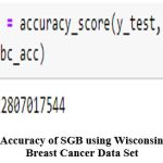Figure 23: Accuracy of SGB using Wisconsin Diagnostic Breast Cancer Data Set   Click here to view Figure

Using the SGB technique, it was discovered that the Wisconsin diagnosis dataset ² had a 96.49% accuracy rate as shown in figure 23while the other breast cancer dataset³ had a 95.62% accuracy rateas shown in figure 22.

Extreme Gradient Boosting

For classification and regression issues, Extreme Gradient Boosting (XGBoost), a powerful machine learning approach, is used. It is a progression of gradient boosting that makes use of a more regularized model to lower over-fitting and increase generalization effectiveness.  Two of XGBoost’s main advantages over traditional Gradient Boosting are its ability to handle very large datasets and its high processing efficiency. This is done by using distributed computing and parallel processing to train several trees at once. A number of additional XGBoost hyper-parameters, such as regularization parameters and learning rate decay, can be changed to enhance the model’s performance. By supporting both tree-based and linear models, it also provides a high level of customization. A key characteristic of XGBoost is its capacity to handle missing data.

Since it can automatically learn how to effectively impute missing values during training, less data preparation is required. Another virtue of XGBoost is its interpretability. The underlying workings of the model can be visualized and understood using a variety of tools, which can be useful for improving and troubleshooting the model. Extreme Gradient Boosting is a reliable and flexible machine learning method that has been shown to produce cutting-edge outcomes on a number of datasets and circumstances. Because of its ability to handle huge datasets, and missing data, and provide interpretability, it is extensively used by data scientists and machine learning specialists. After solving equations 32 and 33, calculate XGBoost.

Where, Residual = Actual value – Predicted value, λ=hyperparameter

After obtaining the Similarity Score for each leaf, the Gain is then calculated using the following equation (33):

Figure 24: Accuracy of XGBoost using Wisconsin Diagnostic Breast Cancer Data Set.   Click here to view Figure

Figure 25: Accuracy of XGBoost using  Breast Cancer Wisconsin (Diagnostic) Data Set   Click here to view Figure

Using the XGBoost technique, it was discovered that the Wisconsin diagnosis dataset ² had a 96.49% accuracy rate as shown in figure 24while the other breast cancer dataset³  had a 97.08% accuracy rateas shown in figure 25.

Cross-Validation

The cross-validation method is used in machine learning to evaluate the performance and generalization of a model. For cross-validation, the dataset is split into k-folds or equal-sized subsets. After training on the first k-1 fold, the model is then tested on the final fold. Through the course of this procedure, which is repeated k times, each fold serves as the test set once. The performance indicators obtained from each fold are then summed to estimate the model’s overall performance. The fundamental advantage of cross-validation is that it provides a more precise evaluation of a model’s performance than a single train-test split. By using a variety of test sets, cross-validation can be used to identify issues like over- or under-fitting and provide a more accurate prediction of how the model will perform on fresh, untested data. Common cross-validation methods include K-fold cross-validation, leave-one-out cross-validation, and stratified cross-validation. The choice of the cross-validation approach is influenced by the particular issue, the size and composition of the dataset, and other factors. In both datasets, the K-fold cross-validation method was applied.

The term “K-fold cross-validation” refers to the division of a dataset into k numbers.  Here, the k-fold cross-validation technique has k iterations. The first k tuples in the first iteration are test elements, while the remaining tuples, k are training elements. The second iteration similarly accepts a sequential k number of components but does not include the test element from the first iteration. When k iterations have been completed, the process is repeated. Find the estimated error for each iteration after that. Due to the fact that every element is equally present in both the training set and the testing set, there are no overlapping concepts in this situation. Calculate the overall estimate error(E) now by using the formula in equation (34) as follows:

Figure 26: Accuracy of Breast Cancer Wisconsin (Diagnostic) Data Set Click here to view Figure

Figure 27: Accuracy of Wisconsin Diagnostic Breast Cancer Data Set   Click here to view Figure

Now that k=10 has been chosen, conduct 10 fold cross validation on both the Wisconsin diagnosis dataset² and the breast cancer dataset ³. Yhe observation is that, a decision tree, SVM, Naive Bayes, KNN, Random Forest, and Logistic regression yielded 0.9359, 0.9670, 0.9652, 0.9670, 0.9651, 0.9651 and 0.9254, 0.9758, 0.9451, 0.9670, 0.9561,0.9802 in breast cancer dataset³   and Wisconsin diagnostic dataset² as shown in figure 26 and 27 respetively. These results are shown in the corresponding result section of Table-2.

Hyper-parameter tuning

The process of choosing the best settings for a machine learning model’s hyper-parameters is known as tuning. Hyper-parameters, such as learning rate, regularization strength, batch size, number of hidden layers, etc., must be specified before to training the model because they cannot be determined immediately from the training data. Because choosing the best settings for hyper-parameters may greatly enhance the model’s performance, hyper-parameter tweaking is crucial. Hyper-parameter tuning is experimenting with various combinations of hyper-parameters and assessing the model’s effectiveness on a validation set. Techniques including grid search, random search, Bayesian optimization, and gradient-based optimization are frequently used in this procedure. It’s crucial to remember that over-fitting might happen if the model is trained on the same data that was used for hyper-parameter tweaking. The dataset is often divided into three sets: a training set, a validation set, and a test set. The validation set is used to fine-tune hyper-parameters, the test set is used to assess the ultimate performance of the model, and the training set is used to train the model. Here used grid search method for hyper parameter tuning.

The optimal set of hyper-parameters for a specific machine learning algorithm can be found using the hyper-parameter tuning technique known as grid search. A grid of all possible hyper-parameter combinations is produced, and each combination is then rigorously examined in order to identify the one that performs the best. The following are the steps for adjusting grid search hyper-parameters:

Definition of the hyper-parameters Determine which of the hyper-parameters our machine learning model wishes to adjust.

Choose the hyper-parameter combination that performed best after evaluating the model’s performance for each combination of hyper-parameters Choose a range of values that will be tested for each hyper-parameter.

By taking the Cartesian product of the hyper-parameter ranges, create a grid of all feasible hyper-parameter combinations.

Each hyper-parameter combination should have a machine learning model trained for it, and its performance should be assessed using a cross-validation method like k-fold cross-validation.

Use the top hyper-parameters discovered throughout the whole training dataset to retrain the machine learning model.

Figure 28: Logistic Regression Accuracy of Breast Cancer Wisconsin (Diagnostic) Data Set after hyper parameter tuning.   Click here to view Figure

Figure 29: SVM Accuracy of Breast Cancer Wisconsin (Diagnostic) Data Set after hyper parameter tuning.   Click here to view Figure

Figure 30 Logistic Regression Accuracy of Wisconsin Diagnostic Breast Cancer Data Set after hyper parameter tuning.   Click here to view Figure

Figure 31: SVM Accuracy of Wisconsin Diagnostic Breast Cancer Data Set after hyper parameter tuning.   Click here to view Figure

Apply SVM and Logistic Regression to both datasets following the creation of the grid search strategy for hyper parameter tweaking. Now, SVM and Logistic Regression offer 0.9802 and 0.9794 accuracy in the Wisconsin Diagnostic dataset² as shown in figure 31 and 30 and they do likewise with 0.9743 and 0.9731 accuracy in breast cancer dataset³  as shown in figure 29 and 28.

ROC Curve

The ROC (Receiver Operating Characteristic) curve is a graphical representation of the performance of a binary classifier at different classification thresholds. It is a widely used assessment metric in machine learning for binary classification problems. The ROC curve is created by plotting the True Positive Rate (TPR) that is also known as sensitivity and False Positive Rate (FPR) that is also known as 1-specificity on the y-axis and x-axis, respectively.

Figure 32: ROC curve   Click here to view Figure

Figure 32 illustrates how the ROC curve is influenced by the sensitivity and specificity of two fundamental factors. False positive rates are plotted on the X-axis of the ROC Curve while true positive rates are plotted on the Y-axis. For the test, the ROC curve may be classified as excellent where the X-axis is 0.90 and the Y-axis is 1, good where the X-axis is 0.45 and the Y-axis is 0.9, acceptable where the X-axis is 0.5 and the Y-axis is 0.8, or fail when the X-axis is 0.3 and the Y-axis is 0.6.

Results

Findings and discussions determine what should be given and how to proceed. Download two datasets for breast cancer prediction: one is the Wisconsin diagnostic dataset², and the other is a breast cancer dataset³ from Kaggle. Eleven different algorithms, including Logistic Regression, Decision Tree, Random Forest, SVM, KNN, Gaussian Naive Bayes, SGD, GBC, SGB, XGBoost, and ANN, may be used with the Wisconsin diagnostic dataset². Ten algorithms, including Logistic Regression, Decision Tree, Random Forest, SVM, KNN, SGD, GBC, SGB, XGBoost, and Gaussian Naive Bayes, are used in total on a second breast cancer dataset³. Each approach delivers accuracy for the two datasets that is essentially the same. However, compared to other methods, SVM offers more accuracy in both datasets. In the Wisconsin diagnostic breast cancer dataset², figure 33 was used to examine the precision of Logistic Regression, Decision Tree, Random Forest, SVM, KNN, Gaussian Nave Bayes, SGD, GBC, SGB, XGBoost, and ANN. In a different breast cancer dataset³, the accuracy of Logistic Regression, Decision Tree, Random Forest, SVM, KNN, SGD, GBC, SGB, XGBoost, and Gaussian Naive Bayes was compared using figure 34.

Figue 33: Accuracy compare in Wisconsin diagnostic dataset2   Click here to view Figure

Figure 34: Accuracy compare in Breast cancer dataset3   Click here to view Figure

Following that, compare the accuracy of the two datasets using each algorithm. Following the use of the K-Fold cross-validation approach, figure 35 shows each algorithm’s accuracy, standard deviation, and run time for the two datasets—the Wisconsin diagnostic dataset² and another breast cancer dataset ³. The optimisation technique Stochastic Gradient Descent (SGD) is typically used to train neural networks and machine learning models. Since each epoch involves several weight update steps and epochs are designed to optimise the learning process, cross validation cannot be used in ANN, SGD,GBS,SBG and XGBoost. Two types of models are used in gradient boosting classifiers, stochastic gradient boosting (SGB), and extreme gradient boosting: a weak machine learning model, generally a decision tree, and a strong machine learning model, made up of several weak models. Cross validation cannot be applied to the Gradient Boosting Classifier, Stochastic Gradient Boosting (SGB), and Extreme Gradient Boosting since it has already been applied to the decision tree.

In figure 35, the Classification and Regression Trees (CART), Support Vector Machines (SVM), Gaussian Naive Bayes (NB), k-Nearest Neighbours (KNN), logistic regression, and random forest algorithms were all cross-validated using the kfold method. After using the k-fold Cross validation approach in both datasets, it is now possible to determine which algorithms offer the maximum accuracy in the first and second places. Apply hyper parameter tweaking to SVM and Logistic Regression as shown in figure 36 as they offer the maximum accuracy in both datasets in this case. After applying the hyper-parameter tuning technique, which is a grid search approach, figure 36 shows that SVM and Logistic Regression offers the greatest accuracy of the two datasets—the Wisconsin Diagnostic dataset² and another breast cancer dataset³.

Figure 35: Accuracy after K-Fold cross-validation   Click here to view Figure

Figure 36: Accuracy after hyper-parameter tuning technique   Click here to view Figure

Compare the SVM maximum accuracy in both datasets after that. When assessing the precision of a predictive model, a binary classifier’s performance is represented graphically as a Receiver Operating Characteristic (ROC) curve.

Figure 37: ROC curve in Wisconsin diagnostic dataset.   Click here to view Figure

Figure 38: G-Mean, and ROC Area of each Algorithm   Click here to view Figure

Every algorithm’s roc curve and roc area in the Wisconsin diagnostic dataset² are described by Figure 37. The ROC areas of the methods Logistic Regression, SVM, Decision Tree, Naive Bayes, KNN, and Random Forest are 0.95, 0.98, 0.94, 0.94, 0.96, and 0.97 respectively. Similar to this, Figure 39 describes the ROC curves for all methods and the ROC regions in a different breast cancer dataset³. The ROC areas of Logistic Regression, SVM, Decision Tree, Naive Bayes, KNN, and Random Forest are 0.95, 0.96, 0.94, 0.95, 0.95, and 0.97 respectively for each method, which are distinct from one another by various colours. A higher G-mean value indicates better performance of the classifier.

Figure 39: ROC curve in Wisconsin diagnostic dataset   Click here to view Figure

Figure 40: G-Mean, and ROC Area of each Algorithm   Click here to view Figure

Discussion

The primary focus of this research is on the algorithm that predicts this cancer with the highest degree of accuracy compared to other algorithms. Use the Wisconsin diagnosis dataset² to apply Decision Tree, Random Forest, SVM, KNN, Naive Bayes, Logistic Regression, SGD, GBC, SGB, XGBoost, and ANN algorithms. Use another breast cancer dataset³ to apply Decision Tree, Random Forest, SVM, KNN, Naive Bayes, SGD, GBC, SGB, XGBoost, Logistic Regression methods. After that, SVM offers the best accuracy in a breast cancer diagnosis dataset from Wisconsin² , while Random Forest and XGBoost offers the highest accuracy in another breast cancer dataset³. Then, use the KFold cross validation approach with both datasets to apply the Decision Tree, Random Forest, SVM, KNN, Naive Bayes, and Logistic Regression algorithms. SVM and Logistic Regression are now shown to have the maximum accuracy in both datasets. Now, for hyper parameter tuning, use the grid search approach on the datasets of both SVM and Logistic Regression. Decide which parameters will work best for the model, then input them. After that, SVM offers the maximum accuracy across both datasets, even when using varied threshold values, G-means, and ROC area. The SVM Threshold value, G-mean value, and ROC area for the Wisconsin diagnostic dataset² is 0.22, 0.98, and 0.98, respectively. The SVM Threshold value, G-mean value, and ROC area is all the same in another breast cancer dataset³, which has a 0.61, 0.97, and 0.96 ROC area. Both datasets are provided with different Threshold values, G-means, and ROC areas by Decision Tree, Random Forest, KNN, Naive Bayes, and Logistic Regression methods, which are described in figure 38 and figure 40.

The best algorithm for predicting this cancer is the major findings of this research. Download two datasets from Kaggle that are connected to this cancer. Now use the KNN, SVM, Naive Bayes, Decision Tree, SGD, GBC, SGB, XGBoost, and Random Forest algorithms on both sets of data. The maximum accuracy is provided by SVM in the Wisconsin diagnosis dataset² and by Random Forest  and XGBoost in a different dataset³ of breast cancer. Utilize the K-Fold cross validation method now on both datasets. Following that, both dataset’s greatest accuracy is provided by SVM and logistic regression. Utilize the hyper parameter tweaking approach now on the SVM and Logistic Regression datasets. Then, in both datasets, SVM has the maximum accuracy. Therefore, it is simple to conclude that SVM is the best method for predicting cancer in any dataset.

SWOT (Strength Weakness Opportunity Threats) Analysis

Strength

Finding an algorithm that offers the best accuracy with the least amount of time and error is the main focus. Hence, use a few machine learning algorithms on two datasets to determine which algorithm has the greatest accuracy. Use the K-Fold cross validation technique and the grid search hyper parameter tuning approach to each algorithm now, and then choose the algorithm that offers the maximum accuracy. Check which algorithm, both before to and during the cross-validation technique and grid search hyper parameter adjustment, delivers the maximum accuracy. In both datasets when all algorithms are applied, SVM therefore offers the maximum accuracy. The optimum technique for predicting any dataset involving breast cancer is hence SVM.

Weakness

A total of eleven methods are used in this research on the Wisconsin diagnostic dataset , although only ten algorithms may be used on another breast cancer dataset due to ANN restrictions.

SVM and Logistic Regression methods in both datasets may be tuned using the hyper parameter approach in this case, while KNN and Decision Tree algorithms cannot. When parameter adjustment is used with KNN and Decision Tree algorithms, accuracy may be higher, lower, or equal to SVM.

Opportunity

In this study, the identical methods are applied to two datasets, and SVM is used on each of them to deliver the maximum accuracy in the shortest amount of time with the lowest error rate. As a result, the healthcare system can readily anticipate whether a patient will get breast cancer or not.

Threats

As machine learning models are trained on a particular dataset, it’s possible that they don’t perform as well in other populations or environments. For instance, when used on a population with different demographics, risk factors, or healthcare practices, a model developed using data from a particular geographic location may not perform as well.

Even while machine learning has a bright future in the field of this cancer prediction, there may not be much of a clinical influence on actual patient care in real-world healthcare settings. The actual application and adoption of these models in standard clinical practice may be influenced by elements including resource accessibility, cost-effectiveness, and clinical workflow integration.

Conclusion

The Wisconsin Diagnostic dataset employed a total of eleven algorithms, whereas another dataset on breast cancer used a total of ten algorithms. In both datasets, our investigation revealed that Support Vector Machine (SVM) produces the best results. According to a prior study, we have discovered that our approach effectively detects this cancer. Although this model employed a total of eleven algorithms, certain breast cancer articles models were constructed using three or four algorithms. This article employs real-time information presentation, making it particularly beneficial for the healthcare system. Whether this cancer is malignant or benign, we can anticipate it using machine learning and artificial intelligence approaches. Results and feature selection are interdependent, thus when the best features are chosen, the model produces the best results, which means it is more accurate. So, if advanced feature selection techniques are developed in the future, the model will offer the greatest accuracy.

The choice of the optimal parameter will enable the model to provide the highest accuracy. Thus, choose a parameter before adjusting the hyper parameter. In the future, if advanced technology is used and advanced hyper parameters are run through the model, the accuracy will be at its greatest in the shortest amount of time with the least amount of mistake.

Acknowledgments

We acknowledge the diverse R&D resources provided by Management, JIS College of Engineering, and JIS GROUP.

Conflict of interest

Authors declare that they have no conflict of interest. This article does not contain any studies with human participants or animals performed by any of the authors. Informed consent was obtained from all individual participants included in the study.

Funding Sources

There is no funding Sources

References

1. Alcohol, tobacco and breast cancer – collaborative reanalysis of individual data from 53 epidemiological studies, including 58 515 women with breast cancer and 95 067 women without the disease – PMC. Published 2023. Accessed September 21, 2023. https://www.ncbi.nlm.nih.gov/pmc/articles/PMC2562507/
2. Breast Cancer Wisconsin (Diagnostic) Data Set. Published 2023. Accessed April 21, 2023. https://www.kaggle.com/datasets/uciml/breast-cancer-wisconsin-data
3. UCI Machine Learning Repository: Breast Cancer Wisconsin (Original) Data Set. Published 2023. Accessed April 21, 2023. https://archive.ics.uci.edu/ml/datasets/breast+cancer+wisconsin+(original)
4. Fan M, Yuan W, Zhao W, et al. Joint Prediction of Breast Cancer Histological Grade and Ki-67 Expression Level Based on DCE-MRI and DWI Radiomics. IEEE J Biomed Health Inform. 2020;24(6):1632-1642. doi:10.1109/JBHI.2019.2956351
   CrossRef
5. Karim MdR, Wicaksono G, G. Costa I, Decker S, Beyan O. Prognostically Relevant Subtypes and Survival Prediction for Breast Cancer Based on Multimodal Genomics Data. IEEE Access. 2019;7:133850-133864. doi:10.1109/ACCESS.2019.2941796
   CrossRef
6. Das S, Mondal D, Majumdar D. Intelligent Application of Laser for Medical Prognosis: An Instance for Laser Mark Diabetic Retinopathy. Biosci Biotechnol Res Asia. 2023;20(2):547-559. doi:10.13005/bbra/3109
   CrossRef
7. Das S, Sanyal MK, Majumdar D, Sanyal M. Artificial Intelligence for Rural Healthcare Management: Prognosis, Diagnosis, and Treatment. In: Mukhopadhyay S, Sarkar S, Mandal JK, Roy S, eds. AI to Improve E-Governance and Eminence of Life: Kalyanathon 2020. Studies in Big Data. Springer Nature; 2023:1-23. doi:10.1007/978-981-99-4677-8_1
   CrossRef
8. Das S, Kundu A, Kumar A, Karmakar B, Saha A. An Intelligent Diagnosis of Adenovirus Disease for Child Healthcare and Prognosis. Indian J Sci Technol. 2023;16(23):1716-1725. doi:10.17485/IJST/v16i23.447
   CrossRef
9. Das S, Sanyal MK, Majumdar D. Correction to: An Intelligent Approach for Detecting COVID-19 Probability. Appl Netw Sens Auton Syst Anal. Published online 2022:C1-C1. doi:10.1007/978-981-16-7305-4_37
   CrossRef
10. Das S, Sanyal MK, Datta D. A Comprehensive Feature Selection Approach for Machine Learning. Int J Distrib Artif Intell IJDAI. 2021;13(2):13-26. doi:10.4018/IJDAI.2021070102
    CrossRef
11. Fatima N, Liu L, Hong S, Ahmed H. Prediction of Breast Cancer, Comparative Review of Machine Learning Techniques, and Their Analysis. IEEE Access. 2020;8:150360-150376. doi:10.1109/ACCESS.2020.3016715
    CrossRef
12. Adnan N, Zand M, Huang THM, Ruan J. Construction and Evaluation of Robust Interpretation Models for Breast Cancer Metastasis Prediction. IEEE/ACM Trans Comput Biol Bioinform. 2022;19(3):1344-1353. doi:10.1109/TCBB.2021.3120673
    CrossRef
13. Peng C, Zheng Y, Huang DS. Capsule Network Based Modeling of Multi-omics Data for Discovery of Breast Cancer-Related Genes. IEEE/ACM Trans Comput Biol Bioinform. 2020;17(5):1605-1612. doi:10.1109/TCBB.2019.2909905
    CrossRef
14. Alghunaim S, Al-Baity HH. On the Scalability of Machine-Learning Algorithms for Breast Cancer Prediction in Big Data Context. IEEE Access. 2019;7:91535-91546. doi:10.1109/ACCESS.2019.2927080
    CrossRef
15. Jebarani PE, Umadevi N, Dang H, Pomplun M. A Novel Hybrid K-Means and GMM Machine Learning Model for Breast Cancer Detection. IEEE Access. 2021;9:146153.
    CrossRef
16. Rawal R. BREAST CANCER PREDICTION USING MACHINE LEARNING. 2020;7.
17. Chauhan A, Kharpate H, Narekar Y, Gulhane S, Virulkar T, Hedau Y. Breast Cancer Detection and Prediction using Machine Learning. In: 2021 Third International Conference on Inventive Research in Computing Applications (ICIRCA). ; 2021:1135-1143. doi:10.1109/ICIRCA51532.2021.9544687
    CrossRef
18. Naji MA, Filali SE, Aarika K, Benlahmar EH, Abdelouhahid RA, Debauche O. Machine Learning Algorithms For Breast Cancer Prediction And Diagnosis. Procedia Comput Sci. 2021;191:487-492. doi:10.1016/j.procs.2021.07.062
    CrossRef
19. Rabiei R, Ayyoubzadeh SM, Sohrabei S, Esmaeili M, Atashi A. Prediction of Breast Cancer using Machine Learning Approaches. J Biomed Phys Eng. 2022;12(3):297-308. doi:10.31661/jbpe.v0i0.2109-1403
    CrossRef
20. Kurian B, Jyothi V. Breast cancer prediction using an optimal machine learning technique for next generation sequences. Concurr Eng. 2021;29(1):49-57. doi:10.1177/1063293X21991808
    CrossRef
21. Das S, Sanyal M. Machine intelligent diagnostic system (MIDs): an instance of medical diagnosis of tuberculosis. Neural Comput Appl. 2020;32. doi:10.1007/s00521-020-04894-8
    CrossRef
22. Das S, Sanyal M, Datta D, Biswas A. AISLDr: Artificial Intelligent Self-learning Doctor. In: Bhateja V, Coello Coello CA, Satapathy SC, Pattnaik PK, eds. Intelligent Engineering Informatics. Vol 695. Advances in Intelligent Systems and Computing. Springer Singapore; 2018:79-90. doi:10.1007/978-981-10-7566-7_9
    CrossRef
23. Das S, Sanyal M, Datta D. Advanced Diagnosis of Deadly Diseases Using Regression and Neural Network: 52nd Annual Convention of the Computer Society of India, CSI 2017, Kolkata, India, January 19-21, 2018, Revised Selected Papers. In: ; 2018:330-351. doi:10.1007/978-981-13-1343-1_29
    CrossRef
24. Sunny J, Rane N, Kanade R, Devi S. Breast Cancer Classification and Prediction using Machine Learning. Int J Eng Res Technol. 2020;9(2). doi:10.17577/IJERTV9IS020280
    CrossRef
25. Asri H, Mousannif H, Moatassime HA, Noel T. Using Machine Learning Algorithms for Breast Cancer Risk Prediction and Diagnosis. Procedia Comput Sci. 2016;83:1064-1069. doi:10.1016/j.procs.2016.04.224
    CrossRef

(Visited 220 times, 1 visits today)