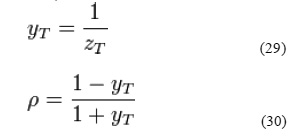
S-parameters refer to the scattering matrix (“S” in S-parameters refers to scattering). The concept was first popularized around the time that Kaneyuke Kurokawa of Bell Labs wrote his 1965 IEEE article Power Waves and the Scattering Matrix. The scattering matrix is a mathematical construct that quantifies how RF energy propagates through a multi-port network. The S- matrix is what allows us to accurately describe the properties of incredibly complicated networks as simple “black boxes”. For an RF signal incident on one port, some fraction of the signal bounces back out of that port, some of it scatters and exits other ports (and is perhaps even amplified), and some of it disappears as heat or even electromagnetic radiation. The S-matrix for an Nport contains a N2coefficients (S-parameters), each one representing a possible input-output path. S- parameters refer to RF “voltage out versus voltage in” in the most basic sense. S-parameters come in a matrix, with the number of rows and columns equal to the number of ports. For the Sparameter subscripts “ij”, j is the port that is excited (the input port), and “i” is the output port. Thus S11 refers to the ratio of signal that reflects from port one for a signal incident on port one. Parameters along the diagonal of the S-matrix are referred to as reflection coefficients because they only refer to what happens at a single port, while off-diagonal Sparameters are referred to as transmission coefficients, because they refer to what happens from one port to another. S-parameters change with the measurement frequency so this must be included for any S-parameter measurements stated, in addition to the characteristic impedance or system impedance. S-parameters are readily represented in matrix form and obey the rules of matrix algebra. Note that each S-parameter is a vector, so if actual data were presented in matrix format, a magnitude and phase angle would be presented for each Sij. The input and output reflection coefficients of networks (such as S11 and S22) can be plotted on the Smith chart. Transmission coefficients (S21 and S12) are usually not plotted on the Smith chart. The Capacitor sometimes referred to as a Condenser is a passive device, and one which stores energy in the form of an electrostatic field which produces a potential (Static Voltage) across its plates. In its basic form a capacitor consists of two parallel conductive plates that are not connected but are electrically separated either by air or by an insulating material called the Dielectric. When a voltage is applied to these plates, a current flows charging up the plates with electrons giving one plate a positive charge and the other plate an equal and opposite negative charge. This flow of electrons to the plates is known as the Charging Current and continues to flow until the voltage across the plates (and hence the capacitor) is equal to the applied voltage Vc. At this point the capacitor is said to be fully charged Units of capacitance is given as below

1µF = 1/1,000,000 = 10-6 F

1nF = 1/1,000,000,000 = 10-9 F

1pF = 1/1,000,000,000,000 = 10-12 F

The factor by which the dielectric increases the capacitance compared with air is known as the Dielectric Constant. The permittivity of the dielectric between the plates is then the product of the permittivity of free space (ε o) and the relative permittivity (ε r) and is given as:

ε = ε 0 * ε r                                               …(1)

Types of capacitor

Capacitors are produced in a wide variety of forms. A fixed-value capacitor has a series of coloured bands around its body, which signifies the capacitor’s value. Variable capacitors are ones whose capacitance can be varied between an upper and lower limit. They may be adjusted by rotary controls and are often used on radio sets to change frequency. ceramic capacitor, electrolytic capacitor, tantalum capacitor, silver mica capacitor, polystyrene film capacitor, polyester film capacitor, metallised polyester film capacitor, polycarbonate capacitor, polypropylene capacitors are the few types available in the industry. Modern capacitors can be classified according to the characteristics and properties of their insulating dielectric Low Loss, High Stability such as Mica, Low-K Ceramic, and Polystyrene. Medium Loss, Medium Stability such as Paper, Plastic Film, High-K Ceramic. Polarized Capacitors such as Electrolytic’s, Tantalum’s.

Scattering parameters

Extremely useful design aid that most manufacturers supply for their higher frequency transistors. S parameters are becoming more and more widely used because they are much easier to measure and work with than Y parameters. They are easy to understand, convenient, and provide a wealth of information at a glance. Historically, an electrical network would have comprised a ‘black box’ containing various interconnected basic electrical circuit components or lumped elements such as resistors, capacitors, inductors and transistors. For the S-parameter definition, it is understood that a network may contain any components provided that the entire network behaves linearly with incident small signals.

It may also include many typical communication system components or blocks such as amplifiers, attenuators, filters, couplers and equalizers provided they are also operating under linear and defined conditions.

S11 = ratio of reflected to incident wave = Return Loss

S21 = ratio of transmitted to incident wave = Insertion Loss

Return Loss represents how much of the signal is reflected back due to any impedance mismatch. The Insertion Loss represents how much of the signal is lost from transferring energy from one port to another; the loss is due to impedance discontinuities and resonance effects of the interconnect.

The S-parameter magnitude may be expressed in linear form or logarithmic form. When expressed in logarithmic form, magnitude has the “dimensionless unit” of decibels. The S-parameter angle is most frequently expressed in degrees but occasionally in radians. S11 refers to the signal reflected at Port 1 for the signal incident at Port

1.Scattering parameter S11is the ratio of the two wave’s b1/a1 shows in figure 4.b

S21 refers to the signal exiting at Port 2 for the signal incident at Port 1.Scattering parameter S21 is the ratio of the two wave’s b2/a1. Diagrametic representation is shown in figure 4.(d) S22 refers to a signal exiting at port 2 for an incident signal at port 2.

S22 is the ratio of b2/a2. S 12 refers to a signal exiting at port 1 for a incident signal at port 2 is shown in figure 5(a). S12 is the ratio of b1/a2.

The transmitted and the reflected wave will have changed in amplitude and phase from the incident wave. Generally the transmitted and the reflected wave will be at the same frequency as the incident wave.

General s-parameter matrix

For a generic multi-port network, each of the ports is allocated an integer ‘n’ ranging from 1 to N, where N is the total number of ports. For port n, the associated S-parameter definition is in terms of incident and reflected ‘power waves’, an bn respectively. Kurokawa defines the incident power wave for each port as

a = 1 / 2 k (v+ZpI)                                 …(2)

and the reflected wave for each port is defined as

b = 1 / 2 k (v-Z*pI)                                …(3)

where Zp is the diagonal matrix of the complex reference impedance for each port, Z*pI is the element wise complex conjugate of Zp, V and I are respectively the column vectors of the voltages and currents at each port and

K = (√R{ Zp }%)-1                                                   …(4)

2-Port S-Parameters

The S-parameter matrix for the 2-port network is probably the most commonly used and serves as the basic building block for generating the higher order matrices for larger networks. In this case the relationship between the reflected, incident power waves and the S-parameter matrix is given by:

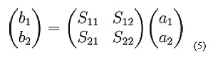
Expanding the matrices into equations gives

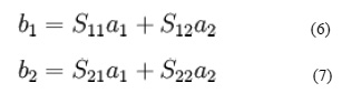
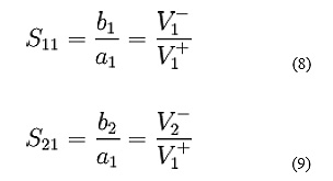
Each equation gives the relationship between the reflected and incident power waves at each of the network ports, 1 and 2, in terms of the network’s individual S-parameters, S11 S12, S21, S22. If one considers an incident power wave at port 1 (a1) there may result from it waves exiting from either port 1 itself (b1) or port 2 (b2). However if, according to the definition of S-parameters, port 2 is terminated in a load identical to the system impedance (Z0) then, by the maximum power transfer theorem, will be totally absorbed making a2 equal to zero. Therefore

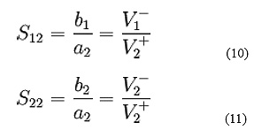
Similarly, if port 1 is terminated in the system impedance then a1 becomes zero, giving

S11 is the input port voltage reflection coefficient.

S12 is the reverse voltage gain.

S21 is the forward voltage gain.

S22 is the output port voltage reflection coefficient.

S-Parameter properties of 2-port networks

An amplifier operating under linear (small signal) conditions is a good example of a non- reciprocal network and a matched attenuator is an example of a reciprocal network. In the following cases we will assume that the input and output connections are to ports 1 and 2 respectively which is the most common convention. The nominal system impedance, frequency and any other factors which may influence the device, such as temperature, must also be specified.

Complex linear gain

The complex linear gain G is given by G = S 21. That is simply the voltage gain as a linear ratio of the output voltage divided by the input voltage, all values expressed as complex quantities. Scalar linear gain: The scalar linear gain or linear gain magnitude is given by %G%=%S 21%. That is simply the scalar voltage gain as a linear ratio of the output voltage and the input voltage.

Scalar logarithmic gain

The scalar logarithmic (decibel or dB) expression for gain (g) is

This is more commonly used than scalar linear gain and a positive quantity is normally understood as simply a ‘gain’… A negative quantity can be expressed as a ‘negative gain’ or more usually as a ‘loss’ equivalent to its magnitude in dB

E. Insertion Loss: Insertion Loss (IL), usually also represented in dB, is given by

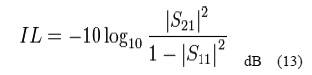
By definition, return loss is a positive scalar quantity implying the 2 pairs of magnitude (|) symbols. The linear part, S 21 is equivalent to the reflected voltage magnitude divided by the incident voltage magnitude.

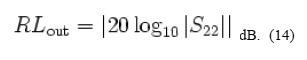
Output return loss

The output return loss (RLout) has a similar definition to the input return loss but applies to the output port (port 2) instead of the input port. It is given by

Voltage reflection coefficient

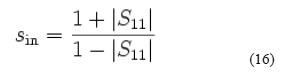
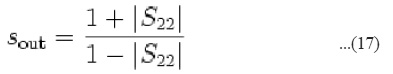
The voltage reflection coefficient at the input port ( Áin ) or at the output port (Áout) are equivalent to S11 and S22 respectively, so Áin = S11 and Áout = S22. Voltage reflection coefficients are complex quantities and may be graphically represented on polar diagrams or Smith Charts. Voltage standing wave ratio (VSWR)

The voltage standing wave ratio (VSWR) at a port, represented by the lower case ‘s’, is a similar measure of port match to return loss but is a scalar linear quantity, the ratio of the standing wave maximum voltage to the standing wave minimum voltage. It therefore relates to the magnitude of the voltage reflection coefficient and hence to the magnitude of either S11for the input port or S22 for the output port.

At the input port, the VSWR (Sin) is given by

At the output port, the VSWR (S out) is given by

 

Four port S-parameters

These are 4×4 matrices having the following s parameters.

Smith chart

The Smith chart, invented by Phillip H. Smith (1905-1987), is a graphical aid or monogram designed for electrical and electronics engineers specializing in radio frequency (RF) engineering to assist in solving problems with transmission lines and matching circuits. Use of the Smith chart utility has grown steadily over the years and it is still widely used today, not only as a problem solving aid, but as a graphical demonstrator of how many RF parameters behave at one or more frequencies, an alternative to using tabular information. The Smith chart can be used to represent many parameters including impedances, admittances, reflection coefficients, scattering parameters, noise figure circles, constant gain contours and regions for unconditional stability. The Smith chart is most frequently used at or within the unity radius region. However, the remainder is still mathematically relevant, being used, for example, in oscillator design and stability analysis.

Actual and normalized impedance and admittance

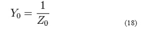
A transmission line with a characteristic impedance of Z0 may be universally considered to have a characteristic admittance of Y0 where

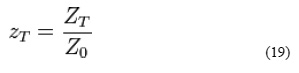
Any impedance, ZT expressed in ohms, may be normalized by dividing it by the characteristic impedance, so the normalized impedance using the lower case z, suffix T is given by

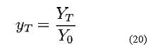
Similarly, for normalized admittance

The SI unit of impedance is the ohm with the symbol of the upper case Greek letter Omega (©) and the SI unit for admittance is the siemens with the Symbol of an upper case letter S. Normalized impedance and normalized admittance are dimensionless. Actual impedances and admittances must be normalized before using them on a Smith chart. Once the result is obtained it may be denormalized to obtain the actual result

The normalized impedance Smith chart

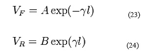
Using transmission line theory, if a transmission line is terminated in an impedance (ZT) which differs from its characteristic impedance (Z0), a standing wave will be formed on the line comprising the resultant of both the forward (VF) and the reflected (VR) waves. Using complex exponential notation:

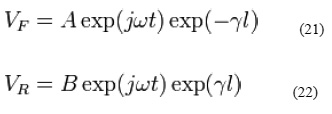
is the temporal part of the wave exp(-ϒl)  is the spatial part of the wave and

ω=2πf  where ω is the angular frequency in radians per second (rad/s)

f is the frequency in hertz (Hz)

t is the time in seconds (s) A and B are constants

l is the distance measured along the transmission line from the generator in meters (m) Also ϒ = α + jβ is the propagation constant which has unit’s 1/m

where

α is the attenuation constant in nepers per meter (Np/m)

β is the phase constant in radians per meter (rad/m)

The Smith chart is used with one frequency at a time so the temporal part of the phase ( ) is fixed. All terms are actually multiplied by this to obtain the instantaneous hase, but it is conventional and understood to omit it. Therefore

Regions of the Z Smith chart

If a polar diagram is mapped on to a cartesian coordinate system it is conventional to measure angles relative to the positive x-axis using a counter-clockwise direction for positive angles. The magnitude of a complex number is the length of a straight line drawn from the origin to the point representing it. The Smith chart uses the same convention, noting that, in the normalized impedance plane, the positive x-axis extends from the center of the Smith chart at

The region above the x-axis represents inductive impedances and the region below the xaxis represents capacitive impedances. Inductive impedances have positive imaginary parts and capacitive impedances have negative imaginary parts. If the termination is perfectly matched, the reflection coefficient will be zero, represented effectively by a circle of zero radius or in fact a point at the centre of the Smith chart. If the termination was a perfect open circuit or short circuit the magnitude of the reflection coefficient would be unity, all power would be reflected and the point would lie at some point on the unity circumference circle.

Circles of constant normalized resistance and constant normalized reactance

The normalized impedance Smith chart is composed of two families of circles: circles of constant normalized resistance and circles of constant normalized reactance. In the complex reflection coefficient plane the Smith chart occupies a circle of unity radius centered at the origin. In cartesian coordinates therefore the circle would pass through the points (1,0) and (-1,0) on the x- axis and the points (0,1) and (0,-1) on the y-axis. Since both Á and are complex numbers, in general they may be expressed by the following generic rectangular complex numbers

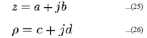
Substituting these into the equation relating normalized impedance and complex reflection coefficient

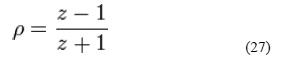
gives the following result:

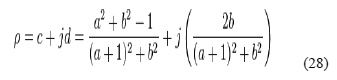
This is the equation which describes how the complex reflection coefficient changes with the normalized impedance and may be used to construct both families of circles.

The Y Smith chart

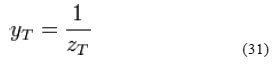
The Y Smith chart is constructed in a similar way to the Z Smith chart case but by expressing values of voltage reflection coefficient in terms of normalized admittance instead of normalized impedance. The normalized admittance yT is the reciprocal of the normalized impedance zT, so

The Y Smith chart appears like the normalized impedance type but with the graphic scaling rotated through , the numeric scaling remaining unchanged. The region above the x-axis represents capacitive admittances and the region below the xaxis represents inductive admittances. Capacitive admittances have positive imaginary parts and inductive admittances have negative imaginary parts.

 

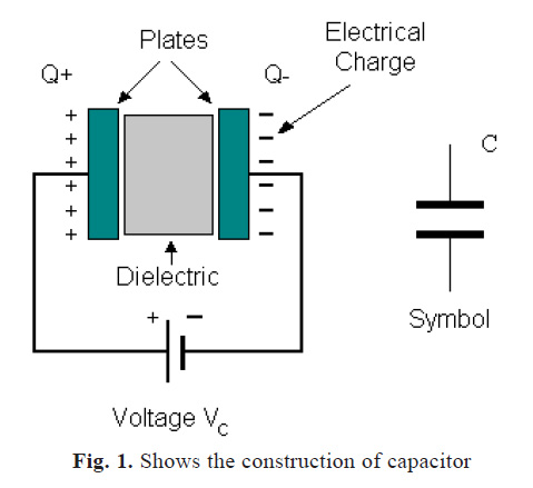Fig. 1. Shows the construction of capacitor Click here to View figure

 

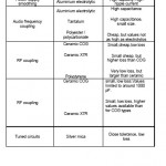Fig. 2. Capacitors uses and applications Click here to View figure

 

Fig. 3. (a) Black Box (b) 2-port network Click here to View figure

 

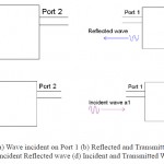Fig. 4. (a) Wave incident on Port 1 (b) Reflected and Transmitted Wave (c) Incident Reflected wave (d) Incident and Transmitted WaveClick here to View figure

 

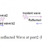Fig. 5. (a) Transmitted Incident reflected Wave at port2 (b) Incident and wave at port 1 Click here to View figure

 

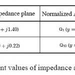Fig. 7. Different values of impedance and admidance Click here to View figure

 

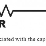Fig. 8. ESR associated with the capacitor Click here to View figure

 

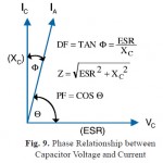Fig. 9. Phase Relationship between Capacitor Voltage and CurrentClick here to View figure

 

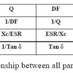Fig. 10. Relationship between all parameters Click here to View figure

 

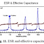Fig. 11. ESR and effective capacitance Click here to View figure

 

The z smith chart and the y smith charts

In RF circuit and matching problems sometimes it is more convenient to work with admittances (representing conductance and susceptances ) and sometimes it is more convenient to work with impedances (representing resistances and reactance). Solving a typical matching problem will often require several changes between both types of Smith chart, using normalized impedance for series elements and normalized admittances for parallel elements. For these a dual (normalized) impedance and admittance Smith chart may be used. Alternatively, one type may be used and the scaling converted to the other when required. In order to change from normalized impedance to normalized admittance or vice versa, the point representing the value of reflection coefficient under consideration is moved through exactly 180 degrees at the same radius.

Values of reflection coefficient, normalized impedances and the equivalent normalized admittances are shown in the below table.

Advantages of the smith chart

The smith chart is a direct graphical representation, in the complex plane, of the complex reflection coefficient. It is a Riemann surface, in that it is cyclical in numbers of half-wavelengths along the line. As the standing wave pattern repeats every half wavelength, this is entirely appropriate. The number of half wavelengths may be represented by the winding number. It may be used either as an impedance or admittance calculator, merely by turning it through 180 degrees. The inside of the unity gamma circular region represents the passive reflection case, which is most often the region of interest. Transformation along the line (if lossless) results in a change of the angle, and not the modulus or radius of gamma. Thus, plots may be made quickly and simply. Many of the more advanced properties of microwave circuits, such as noise figure and stability regions, map onto the SMITH chart as circles. The “point at infinity” represents the limit of very large reflection gain, and so therefore need never be considered for practical circuits. The real axis maps to the Standing Wave Ratio (SWR) variable. A simple transfer of the plot locus to the real axis at constant radius gives a direct reading of the SWR. Characterization of capacitors

The capacitor is normally characterised by the ESR (Equivalent series Resistance), Quality Factor, Dissipation Factor, Tangent Loss and the capacitive reactance etc..

Equivalent series resistance

All physical devices are constructed of materials with finite electrical resistance, which means that physical components contain some resistance in addition to their other properties. All capacitors have a certain amount of resistance to the passage of AC current; this resistance is typically modeled as a resistor in series with a “perfect” capacitor. The value of this resistor is the ESR. ESR is frequency dependent.

Electrolytic capacitors have a tendency to increase in ESR over time due to drying out or corrosion. This increase in ESR has particularly been noted as a problem in switching power supplies. The increase in ESR increases both voltage drops within the capacitor and the heat produced in the caps due to resistive heating. ESR

– Equivalent Series Resistance, DF – Dissipation Factor, and Q or Quality factor are three important factors in the specification of any capacitor. They have a marked impact on the performance of the capacitor and can govern the types of application for which the capacitor may be used. There are two common causes of high ESR:

1) Bad electrical connections

2) Drying of the electrolyte solution.

Electrical connection problems can happen in old or new capacitors, while drying is usually only a problem in old ones. Connection problems happen because the leads coming into the capacitor cannot be made of aluminium, since aluminium cannot be soldered. Drying problems occur because of the importance of water in the electrolyte solution. The solution soaks the paper spacer between the two aluminium plates. The water carries the electrical charge from the negative aluminium plate to the surface of the insulating oxide on the positive plate. The oxide forms the capacitor’s dielectric and the negative charge on the surface of the oxide forms the negative capacitor plate. As the water evaporates, the electrical resistance increases.

Quality factor

There are two separate definitions of the quality factor that are equivalent for high Q resonators but are different for strongly damped oscillators. Generally Q is defined in terms of the ratio of the energy stored in the resonator to that of the energy being lost in one cycle

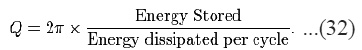
The factor of 2À is used to keep this definition of Q consistent (for high values of Q)

with the second definition

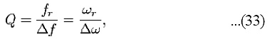
where fr is the resonant frequency, ”f is the bandwidth, Ér is the angular resonant frequency, and ”É is the angular bandwidth. The definition of Q in terms of the ratio of the energy stored to that of the energy dissipated per cycle can be rewritten as:

Where w is defined to be the angular frequency of the circuit (system), and the energy stored and power loss are properties of a system under consideration. The Q of a capacitor is important in tuned circuits because they are more damped and have a broader tuning point as the Q goes down.

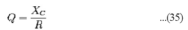
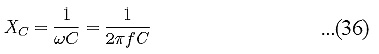
Where XC is the capacitive reactance.

Q is proportional to the inverse of the amount of energy dissipated in the capacitor. Thus, ESR rating of a capacitor is inversely related to its quality.

Dissipation factor

The inverse of Q is the dissipation factor (tan (δ)). Thus, tan (δ) = ESR/XC and the higher the ESR the more losses in the capacitor and the more power it dissipate. If too much energy is dissipated in the capacitor, it heats up to the point that values change (causing drift in operation) or failure of the capacitor.

Where δ is the angle between the capacitor’s impedance vector and the negative reactive axis. XC is the capacitive reactance.

Relationship between ESR, Q, DF and XC

The following figure shows the phase relationship between capacitor voltage and current as well as dissipation factor, ESR, and magnitude of the impedance. In the ideal capacitor the current leads the voltage by 90 degrees. IA in the diagram below denotes the actual current flow through the capacitor and forms angle ´ referred to as the loss angle. Also note that the relationship between IA and Vc is proportional to the relationship between Xc and ESR. The general rule is that DF is factor that is most useful when designing for applications operating at frequencies below

1MHz where the main loss factor is attributable to dielectric loss. ESR and the associated Q value are virtually always associated with metal losses at higher radio frequencies. Power dissipation

The power dissipated in a capacitor can be calculated by multiplying the ESR by the square of the RF network current. Power dissipation in the capacitor is therefore expressed as

Power Dissipation = ESR x (RF current)2 OR

pd = ESR * I2

Polymer dielectric materials

There are variety of dielectric material has been used in the capacitors in the Electronics industry. Out of which the polymer based dielectric material product has made a great impact. The Polypropylene dielectric capacitors now occupy a unique position in both the AC and DC capacitor world. This versatile dielectric features a low dissipation factor that makes it good for AC applications. It also exhibits a high insulation resistance and a low dielectric absorption, which makes it ideal for the precision DC capacitor world.  The maximum service temperature of this film is 105°C.Polypropylene capacitors are now firmly established in the capacitor world. Not all product lines are suited for every application. The product data sheets should be checked for variations.

Capacitance

Shall be within specified tolerance when measured at or referred to 1000 ±20 Hz for values up to and including 1.0 MFD at 25° 5°C.Capacitance values greater than 1.0 MFD shall be measured or referred to 120 ±20 Hz.

Dissipation Factor

Shall not be greater than .1% when measured at or referred to 1000 ±20 Hz for values up to and including 1.0 MFD at 25° ±5°C. Capacitance values greater than 1.0 MFD shall be measured or referred to 120 ±20 Hz.

Dielectric Strength

200% rated voltage for one minute through a limiting resistance of 100 ohms/volt at 25°C.

Temperature Range

-55° to +105°C at full rated voltage. AC types may require temperature derating to allow for self-heating.

Applications

Polypropylene capacitors can be used in a variety of applications. Their low losses (dissipation factor) make them a natural for AC applications. They are well suited for high power applications such as switching power supplies. Attention to the temperature and curent limitations is essential. They are well behaved with frequency and are usable up to the resonant frequency of the capacitor. The ESR parameter is important in limiting self-heating and should be used for product characterization f parts intended for such applications. The ability to operate under corona onset characteristics makes them desirable for a number of AC power applications. In either case, the capacitor construction is optimized for its intended application. Usage outside of this application should be done with caution and forethought. Due to their exceptional stability and environmental performance, polypropylene capacitors are useful in precision applications and are recommended when close tolerance is needed. Filtering, timing, sample and hold, integration and similar precision applications are ideally suited for polypropylene. They are also ideal in audio applications and provide superior sound fidelity when used in coupling equalization or speaker crossover circuits.

Proposed methodology

The new proposed methodology capacitor consists of Re-cycled (R-pet) Poly ethylene terepthalate of closite15A, closite25A, and closite30B has taken into account. This sample results were compared with the existing polypropylene capacitors. Recycled poly (ethylene terepthalate), R-PET, was mixed with organically modified quaternary alkyl ammonium montmorillonite in the contents of 1, 2, and 5 weight %. Three types of clays were evaluated during this work. For comparison, 2 weight % clay containing samples were prepared with three different clay types, Cloisite15A, 25A, 30B.A. The recycling of poly ethylene terepthalate (RPET) : PET, polyester, has been known for many years since the first laboratory samples of this fiber were developed by a small English company in 1941. Then, this research was enlarged by the findings of Dupont on textiles in the 1950s, and the work of Goodyear introducing the first polyester tire fabric in1962s. In the late 1960s and early 1970s, polyesters were developed specifically in the area of packaging- film, sheet, coatings and bottles. The recycling of PET soft drink bottles began soon after their introduction in 1977. Over the past decades, the technology for recycling PET soft drink bottles has been advancing. Though the most commercial recycling systems, like water bath/hydro cyclone, solution/washing, and solvent/flotation processes depending on some flotation or hydro cyclone processes to separate the PET from HDPE base cup-resin, have been developed. The commercial types of recycling systems were designed to process PET at the rate of 10-40 million pounds (4-18×103 tons) per year.

Organoclays

Experiments were carried out with three different types of montmorillonites,  namely Cloisite 30B, 15A, and 25A. These organoclay structures show differences in selection according to what degree of polarity they have. There is an increase in relative product hydrophobicity and a decrease in product polarity in the order of 30B, 25A, and 15A. The hydrophobicity resulted from different natures of organic modifiers affects the chemical compatibility between the polymer and the filler.

Result analysis

The S-parameter analysis for the new dielectric materials to obtain the key performance parameters such as gain, stability, reflection loss, matching impedances has been plotted. Parameters may be displayed as either a rectangular plot, on a Smith chart or polar plot, or as a tabular listing of numeric results. In this section the results of the existing polypropylene capacitor is compared with the new dielectric materials of
cloisites 15A, 25A, 30 dB

CONCLUSION
The newly proposed methodology of a Polyester based Recycled Poly Ethylene terephthalate (R-PET),is taken as the base material and it is mixed with various materials called Cloisite 15A, 25A and 30B.The new composites (di-electric) material have been produced with the ratio of 1wt%,2wt% and 3wt% as seen in the earlier chapter . According to the newly made materials various analysis like Impedance match (Z), scattering parameters like S11, S12, S22, S21, Equivalent Series Resistance, and Effective Capacitance and also the quality factor has been performed and their results have been discussed in the result analysis. The electrical properties of the Dielectric constant, has been excellent when compare with the existing methodology of the polypropylene capacitors. The three samples namely Cloisite 15A, 25A, 30B results were compared with the standard Polypropylene (PP) Capacitor to decide the performance of the new dielectric material. When comparing with the smith chart analysis the chart comparison states that the (R-PET+ 2wt %) Cloisite 30B is a good Nano Capacitor. The Cloisite 30B can work in the frequency range of 0.4GHz to 14.5GHz when compare with the other two materials.

REFERENCES

1. Gonzalez, Guillermo (1997); Microwave Transistor Amplifiers Analysis and Design, Second Edition; Prentice Hall NJ; pp 212-216. ISBN 0-13-254335-4
2. Wiley High Frequency Techniques – AnIntroduction to RF and Microwave Engineering
3. Rf Circuits Design Theory and Applications
4. Smith Chart Basics Microwave Encyclopedia Microwaves101.com
5. Capacitor ESR, Dissipation Factor, Loss Tangent and Q Radio-Electronics.Com
6. How to Measure S-Parameters htm
7. ESR-df-loss-tangent-q-tutorial-basics.php.htm
8. Smith chart – Wikipedia, the free encyclopedia
9. Q factor – Wikipedia, the free encyclopedia
10. Capacitors and ESR – Transwiki
11. S-Parameter_Files.htm
12. The smith chart.htm
13. Capacitor types and their uses

(Visited 1,074 times, 1 visits today)