Introduction

The quantitative examination of ligament morphometric properties from attractive reverberation imaging (MRI) is turning into the standard strategy these days for appraisal of joint ailment, for example, rheumatoid joint inflammation, osteoarthritis et cetera. These are extremely significant devices for assessment of joint illness movement and observing of treatment.^1,2,3 MR imaging is the most favored strategy for ligament imaging as a result of its non – intrusiveness, high delicate tissue difference and its multi-planar and three-dimensional information procurement.^2,3 However in MRI the tissues with close dim level, for example, ligaments may show up as various powers. Likewise the utilization of just a solitary heartbeat grouping for ligament division confines the measure of automatization accomplished. Besides, it has been demonstrated that a solitary heartbeat grouping is not adequate for the precise assessment of the phase of osteoarthritis in knee joint.^4,5,8

In spite of the fact that these new systems can possibly be connected into extensive populace thinks about, a large portion of them requires exceedingly prepared clients to accomplish the ideal execution; accordingly, constraining their relevance. This prerequisite can be limited by the advancement of more robotized division calculations. Likewise theautomatization can furnish MR pictures with great difference and high spatial determination.⁵ Besides, the movement of PC illustrations has permitted the formation of capable altering apparatuses that has streamlined the intelligent division required by semi-robotized approaches like the one displayed in this work. In this manner goal of the present review is to outline a quick and precise articular ligament division system which is the most imperative essential for exact ligament thickness estimation. The achievement of any ligament ensuring and restoring convention relies on precisely deciding the ligament thickness which is the crucial markers of joint sicknesses.^8,9

Literature Review

The watershed transform has been widely used in many fields of picture handling, including medicinal picture division. Due to the number of favorable circumstances that it has: it is a straightforward, natural and quick technique that can be parallelized (a practically direct speedup was accounted for various processors up to 645), and it creates an entire division of the picture in isolated areas regardless of the possibility that the difference is poor, along these lines staying away from the requirement for any sort of form joining. Moreover, a few specialists have proposed strategies to implant the watershed change in a multi scale system, in this manner giving the upsides of these portrayals.⁸

“In a review performed by Ghosh et al. (2000), a low pass channel based concealing was connected to make up for the inhomogeneous loop gathering profile. Inundation based watershed calculation driven by variety in pixel power, spatial nearness and location of territorial minima and bunching – was connected to each veiled picture volume to play out the essential division errand.⁸ A lexible” circle based, iterative separation minimization calculation was executed for ligament thickness dissemination. For intra/entomb gather correlation, volumes of the patellar, tibia1 and femoral ligament were standardized by the epicondylar separate (ED), a parameter invariant to OA.Edges can be identified utilizing different edge finders. These incorporate Sobel, Prewitt, Roberts, Laplacian of Gaussian (LoG), Zero intersections and Canny. In this paper we have utilized LoG to recognize the edge of the picture. The watershed change is an intense morphological instrument for picture division. Tragically, the watershed division procedure prompts an over division issue .^10,11 Beucher and Lantuejoul were the first to apply the idea of watershed to computerized picture division issues. A decent number of works has as of now been done on watershed division and these are accessible in the distributed or online writing.^12,13 The Laplacian of Gaussian edge recognition administrator is utilized with the watershed calculation to produce the last division comes about with less over division.¹⁵ The slope greatness of a picture is considered as a topographic surface for the watershed change. Watershed lines can be found by various ways. The entire division of the picture through watershed change depends for the most part on a decent estimation of picture angles. The consequence of the watershed change is corrupted by the foundation clamor and creates the over-division. Additionally, under division is created by low-differentiate edges produce little size angles, making particular areas be mistakenly combined.¹⁴ A watershed change as a way to isolating covering objects. We can consider the picture as a scene or topographic help where the dim level of every pixel is deciphered as its height in the alleviation. Drenching the scene in a lake with gaps penetrated in nearby minima, catchment bowls will top off with water beginning at these neighborhood minima. At focuses where water originating from various bowls would meet, dams are fabricated. This procedure closes when the water level has achieved the most astounding top in the scene. Therefore, the scene is apportioned into locales or bowls isolated by dams, called watershed lines or just watersheds.¹⁶ The watershed is connected to the picture slope and the watershed lines isolate homogeneous districts, giving the coveted division result. The slope picture for the change is regularly discovered utilizing the morphological angle. Be that as it may, clamor in the inclination picture brings about over-division which can have a critical antagonistic effect on the nature of the division comes about. The nature of the inclination assess impacts them division execution.¹⁷ So the consequence of various slopes on watershed has been found with the assistance of pinnacle flag to commotion ratio. The watershed change normally prompts over division of pictures because of picture clamor and other neighborhood anomalies. To defeat this, inquires about have proposed numerous techniques, for example, marker controlled watershed division, various leveled division and multiscale division. Because of number of focal points watershed change has been generally utilized as a part of many fields of picture preparing. This strategy is the morphological based picture division. This strategy create a total division of the picture in isolated locale regardless of the possibility that the differentiation is poor, along these lines maintaining a strategic distance from the requirement for any sort of form joining.¹⁸

Human Knee joint is made out of femoral head femur and tibia. The surface between femoral head and the internal surface of tibia are secured with a layer of ligament tissue, with the synovial liquid filled between two layers of ligament as ointment.  More often than not in the MR pictures, it’s hard to recognize layers of ligament since they coordinate nearly. By footing innovation to extend knee joint, the femoral head and femoral ligament can be seen unmistakably in MR pictures. Figure 1 indicates MR projective picture of a knee joint after footing, and articular ligament in the figure is shown as a high-brightness [Fig-1]. Expansion to the femoral head and femora ligament, some of encompassing delicate tissue and commotion are additionally appeared as a high shine.

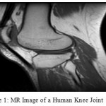Figure 1: MR Image of a Human Knee Joint   Click here to View figure

The upsides of the watershed change are that it is basic, instinctual information, and can be parallelized. The primary disadvantage of this strategy is the over-division because of the nearness of numerous nearby minima. The disadvantage is here remunerated by joining this change with a checking performed. The inside marker is resolved naturally by joining systems including Canny edge location, thresholding and morphological operation. The principle goal of this paper is to discover the crevices in existing writing. The diverse division systems are looked into and found that marker based is best in the greater part of cases since it denote the areas then section them. In any case, advancing the checking locales is as yet a region of research.

Methodology

Image Acquisition and Pre Processing

MR pictures were taken from knee joint of elderly females (>50 years) using brisk destroyed slant resound course of action to projective picture in the sagittal and coronal orientation of the knee joint using 1.5Tesla High Definition Edge MR structure (Manufactured by GE). Projective imaging parameters were according to the accompanying: repetition time(TR)/reverberate time(TE)= 10.4/4.8 ms; flip point = 15º; field of view(FOV)= 160 mm x 160 mm; cross section = 256 x 256; fragment thickness = 1.6 mm; number of signs picked up = 2; getting time = 4 min 38 s.

Picture pre-get ready included presentation, smoothing and overhaul. The photo inclusion was executed to redesign the exactness of picture division, which improved the assurance from 256 x 256 to 399 x 376 for sagittal and 368×361 for coronal picture and making the measure of each photo pixel change from 0.625mm x 0.625mm to 0.3125mm x 0.3125mm. Figure 2 and 3 shows the sagittal and coronal pictures of knee joint after contribution.

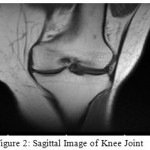Figure 2: Sagittal Image of Knee Joint   Click here to View figure

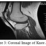Figure 3: Coronal Image of Knee Joint   Click here to View figure

In this work types of images coronal and sagittal planes are used and the process applied to both the images are 100% similar in spite of some changes of about 5% due to the orientation of the Knee in sagittal and coronal planes and morphological operation applied to them. The images were taken in MATLAB and converted from type RGB to Grayscale so that it is comfortable to work with the single pixel values instead of three.

Images pre-processing was carried out so as to make it easy to work with.For this, 1.Filtering: The image is filtered from unwanted noise by using 2-D median filtering operator. 2.Cropping:The images are cropped in order to focus the process on the area of interest by conventional cropping function (imcrop by size-116×174 approx.) 3. Resizing or Interpolated: The images were interpolated (Bi-cubic Interpolation) by imresize function to have 1.5 times bigger (174×261 approx. acc. to cropped image size) version of image and finally 4. Sharpening: The images were sharpened with the imfilter function using appropriate inbuilt filters or convolution kernel.

Image Segmentation for Area of Interest

Harsh Segmentation Using Watershed Algorithm

Watershed Algorithm: Consider two topographic surfaces. Water would gather in one of the two catchment bowls. Water falling on the watershed edge line isolating the two bowls would probably gather into both of the two catchment bowls. Watershed calculations at that point discover the catchment bowls and the edge lines in a picture. The calculation fills in as takes after: Suppose a gap is punched at each territorial nearby least and the whole geology is overwhelmed from underneath by giving the water a chance to ascend through the gaps at a uniform rate. Pixels underneath the water level at a given time are set apart as overwhelmed. When we raise the water level incrementally, the overwhelmed locales will develop in measure. Inevitably the water will ascend to level where two overflowed areas from isolated catchment bowls will blend. At the point when this happens, the calculation builds a one-pixel thick dam that isolates the two districts. The flooding proceeds until the point when the whole picture is fragmented into discrete catchment bowls partitioned by watershed edge lines. Figure 4 shows how watershed segmentation algorithm works on image [Fig-4].

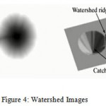Figure 4: Watershed Images   Click here to View figure

Removing Noise in Rough Segmentation by Morphological Operations

The areas in the binary image which are not desired are considered as the noise areas and these are to be removed from the binary image. These areas are of two types: smaller than the desired area (in sagittal and coronal both) and larger than the desired (in sagittal image). So these noisy areas are removed by using the process of dilation and erosion with the morphologically opening binary image using area open function (removing small object)-[5].The larger noise areas are first to be detected and then to be removed separately from binary image.¹³ After removing these entire noisy regions desired region is produced.¹¹

Accurate Edge Extraction and Segmentation

The  Shrewd edge marker is the essential subordinate of a Gaussian and almost approximates the head that enhances the aftereffect of banner to-bustle extent and imprisonment. The Shrewd edge area estimation is consolidated by the going with documentation.

Let I[i, j] denote the image. The result from convolving the image with a Gaussian smoothing filter using separable filtering is an array of smoothed data,

S[i, j] = G[i, j;α ]* I[i, j],

Where α is the spread of the Gaussian and controls the degree of smoothing. The gradient of the smoothed array S[i, j] can be computed using the 2 x 2 first-difference approximations to produce two arrays P[i,j] and Q[i,j] for the x and y partial derivatives:

P[i,j] ~ (S[i,j + 1]- S[i,j] + S[i + 1,j + 1]- S[i + 1,j])/2

Q[i,j] ~ (S[i,j] – S[i + 1,j] + S[i,j + 1]- S[i + 1,j + 1])/2.

The limited contrasts are found the middle value of over the 2×2 square so that the x and y fractional subsidiaries are processed at a similar point in the picture. The greatness and introduction of the inclination can be registered from the standard recipes for rectangular-to-polar transformation:

Q[i,j]=arctan(Q[i,j],P[i,j])

Where the arctan work takes two contentions and creates an edge over the whole hover of conceivable headings. These capacities must be figured effectively, ideally without utilizing drifting point math. It is conceivable to register the inclination size and introduction from the incomplete subsidiaries by table query. The arctangent can be registered utilizing for the most part settled point arithmetic2 with a couple of basic drifting point figurings performed in programming utilizing number and settled point math. Sedgwick gives a calculation to a whole number estimation to the inclination edge that might be adequate for some applications.

Now the canny edge detection process was applied on the binary image produced from the last process in order to detect the boundary of the segmented object in the binary image[3].Now applying these boundaries in the original image by superimposing the canny edge boundary image on the original grayscale image by proper pixel manipulation in these images[1]. At last final segmented Region is highlighted by showing the corresponding pixels of the object (in binary image) on the actual grayscale image and making the other pixels of single same non-highlighted value.¹⁸ The final image is desirably segmented.

Result and Discussion

The proposed systems were produced in MATLAB R2010a conditions. The trials were performed on a PC (I3 Processor: 3 GHz; RAM: 2 GBytes; HD:220GBytes). The execution of the created procedure was assessed on 20 real MRI Images of Knee joints and just aftereffects of agent pictures are exhibited in this review. The results of the study were compared with the actual result of the same knees and found the similarity was above 85%. The thickness of the cartilage is calculated by obtaining the pixel distance from tibia and femur and then calibrating it with proper value.Comparison is made with the diagnostic reports and images.

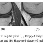Figure 5a: Noise sifted picture of sagittal plane, (B) Cropped Image of sagittal plane, (c) Resize of edited picture 1.5 times in sagittal plane and (D) Sharpened picture of sagittal plane Click here to View figure

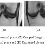Figure 6a: Noise sifted picture of coronal plane, (B) Cropped Image of coronal plane, (c) Resize of trimmed picture 1.5 times in coronal plane and (D) Sharpened picture of coronal plane   Click here to View figure

We actually apply the two process of segmentation here one after the other that is the watershed algorithm segmentation [Fig-9,10] process and the little amount of the morphological operations with the canny edge detector [Fig -13,14,15] at the final segmentation process. If morphological operations [Fig- 7,8] in this segmentation are considered they may prone to some variation with the original image they can change the pixel values from 5-15% which lead to the error result of about 5-10%. Here in the operations of Erosion and dilation there are some pixel disturbances from that of original. This can be calculated by calculating the number of pixels diversions from the original or desired area of the thickness and then this value can be considered as a parameter to judge the errors in the image or may be represented as percentage by a ratio of val(no. of pixel diverted/no. of pixels in desired area to be segmented).

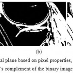Figure 7a: Binary image of sagittal plane based on pixel properties, (b) Dilated version of the binary image extracted previously (c) 1’s complement of the binary image obtained previously   Click here to View figure

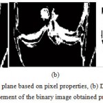Figure 8a Binary image of coronal plane based on pixel properties, (b) Dilated version of the binary image extracted previously (c) 1’s complement of the binary image obtained previously   Click here to View figure

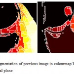Figure 9: Watershed segmentation of previous image in colourmap‘HOT’(a) sagittal plane (b) coronal plane   Click here to View figure

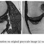Figure 10: Watershed segmentation on original grayscale image (a) sagittal plane (b) coronal plane   Click here to View figure

Another limitation of the present work is that it can only be performed on the predefined types of images or it may give error result if operated on another type of MRI machine with different illumination factor by changing segmentation of the image by about 2-3%. In these cases the Segmentation process described ceases to give the accurate results. Sometimes the shape and structure of the bones and cartilages in the knee joint may also be responsible for the error for about 1-2% in the accurate reading and processing of the pixel in the prescribed algorithm.¹ Now considering the positive side of the segmentation work it will gives the 90-95% accurate results under the given circumstances prescribed in the work.

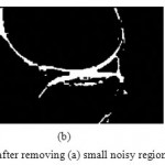Figure 11: Binary image of sagittal plane after removing (a) small noisy regions (b) Large noisy regions (c) all the noise   Click here to View figure

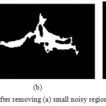Figure 12: Binary image of coronal plane after removing (a) small noisy regions (b) Large noisy regions (c) all the noise   Click here to View figure

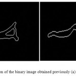Figure 13: Canny edge detection of the binary image obtained previously (a) sagittal plane (b) coronal plane   Click here to View figure

We tentatively demonstrated that the proposed strategy within the sight of the accessible informational indexes indicated viable in 93.5% of the slices. The disappointment of the calculation in the rest of the cuts was for the most part because of poor imaging condition, inadequate footing, and inconsistency in the round state of hard and ligament tissues. In such cases, even the judgment of a specialist in deciding the correct area of the articular space was dubious. We have to assess the calculations with more informational collections, coordinate the proposed procedure in a product bundle for ligament division, ligament thickness delineate and relating 3D perceptions.

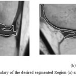Figure 14: Outlining the boundary of the desired segmented Region (a) sagittal plane (b) coronal plane   Click here to View figure

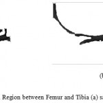Figure 15: Desired segmented Region between Femur and Tibia (a) sagittal plane (b) coronal plane    Click here to View figure

Later on we will research how the power in homogeneities in the MRI information can be managed. We are as of now analyzing the utilization of a consolidated dynamic shape model of the femur and tibia to expand the power and exactness of the bone division. At present, our outcomes show that some manual post-preparing is as yet required to draw level with human-rater execution. Notwithstanding, we are sure that with our proposed system and the recommended upgrades we will have the capacity to build the quantity of situations where manual post processing will end up plainly old.

Conclusion

To finish modified femoral tendon with space among femur and tibia division on MR picture, a customized division procedure in light of Watershed Algorithm and flexible insightful edge revelation has been proposed. Expansion, smoothing and update were completed in the photo pre-get ready to improve the photo quality. The region of interest was picked and the target area for the brutal division was understands by considering the anatomical structure basic (Pixel qualities) of Knee joint. Watershed Algorithm was used to by and large part the photo for the gap amidst femur and tibia. Additional isolating through Morphological operations-picture extension and breaking down with parallel picture opening limits is then associated with clear riotous zones to definitely part the required area from the by and large separated region. Picture checked and filtered in a custom one by one approach to empty the uproarious territories ones and secure the right inner and outside edges of the space among femur and tibia. Edges in the offensive territory were isolated out by as far as possible quick edge locator. As shown by the properties of the pixel on recognized edge, these edges and combined picture were then used to highlight the genuine divided area in the genuine grayscale. Finally the correct division was expert by removing the photo data in the highlighted Region. Division investigate favors the strategy. The whole procedure did not require manual intervention and the adequacy of division handle was advanced. This modified division procedure is successfully associated for both the plane i.e. sagittal and coronal.

Acknowledgements

This research was supported by the Sarkar Diagnostic and Hind Hospital, Lucknow. We thank them for technical aid and providing data for this research.

References

1. Jose G., Tamez-Pena, Monica Barbu-McInnis and Saara Totterman Virtual Scopics, “Knee Cartilage Extraction and Bone-Cartilage Interface Analysis from 3D MRI Data Sets”  350 Linden Oaks, Rochester NY, 14625, USA,2004.
2. Cao Y., Liu X., Cao Y and Yu-nan L. Automatic Segmentation of Femoral Cartilage from MR Image Based on Hough Transform and Adaptive Canny Detection. International Journal of Signal Processing, Image Processing and Pattern Recognition. 2013;6:4.
3.  Sato Y., Nishiif T.,  Nakanishi K.,  Tanaka’ H., Sugano N.,Yoshikawa H., Nakamurat H.,  Visual T. S.,Khanmohammadi M., Zoroofi R. A. Automated Segmentation of the Articular Space in MR Images of the hip joint”  Information Engineering,IET International Conference. 2006.
4.  Wang Y.,Wluka E. A., Jones G.,  Ding C and Flavia M. Use magnetic resonance imaging to assess articular cartilage   Cicuttini. Therapeutic Advances in Musculoskeletal Disease. 2012;4(2):77–97. DOI: 10.1177/ 1759720X11 431005.
5.  Carballido-Gamio J., Lee K.,  Ozhinsky E., Majumdar S.  MRI cartilage of the knee segmentation analysis and visualization. United State.Proc. Intl. Soc. Mag. Reson. Med.  2004;11.
6.  Seim H., Kainmueller D., Lamecker H.,Bindernagel M.,  Malinowski J andZachow S. Model-based Auto-Segmentation of Knee Bones and Cartilage in MRI Data”, 14195 Berlin, Germany,2010.
7. S. Martelli, V. Pinskerova,“The shapes of the tibial and femoral articular surfaces in relation to tibio femoral movement” From the Rizzoli Orthopaedic Institute, Bologna, Italy and the Orthopaedic Clinic, Prague, Czech Republi,J Bone Joint Surg [Br], 84-B:607-13,2002.
   CrossRef
8. S. Ghosh, Beuf, D. C. Newitt, M. Ries, N. Lan and S. Majumda.“Watershed Segmentation of High Resolution Articular Cartilage Images for Assessment of OsteoArthritis”,Proceedings of the 22nd Annual International Conference of the IEEE Engineering in Medicine and Biology Society (Cat. No.00CH37143), Chicago, IL, vol.4, 2000, pp. 3174-3176.
9. “Improved Watershed Transform for Medical Image Segmentation Using Prior Information”  V. Grau*, A. U. J. Mewes, M. Alcañiz, Member, IEEE, R. Kikinis, and S. K. Warfield, Member, IEEE Transactions on Medical Imaging, Vol. 23, No. 4, April 2004.
10. S. Thilagamani, N.Shanthi, “A Novel Recursive Clustering Algorithm for Image Oversegmentation”, European Journal of Scientific Research, Vol.52, No.3, pp.430-436, 2011.
11. Peter Eggleston, “Understanding Oversegmentation and Region Merging”, Vision Systems Design, December 1, 1998.
12. M. W. Hansen and W. E. Higgins, “Watershed-based maximum-homogeneity filtering,” IEEE Trans. Image Process., vol. 8, no. 7, pp. 982-988, Jul. 1999.
    CrossRef
13. K. Parvati, B. S. PrakasaRao and M. Mariya Das, “Image Segmentation Using Gray-Scale Morphology and Marker-ControlledWatershed Transformation”, Discrete Dynamics in Nature and Society,vol. 2008, pp. 1-8, 2008.
    CrossRef
14. Dr.(Mrs)S.N Geethalakshmi and T.Jothi, ”Segmentation Based On Enhanced Morphological Watershed Algorithm”, Journal of Global Research in Computer Science,Volume 1, No. 4, November 2010.
15. P.P.Acharjya1, A. Sinha2, S.Sarkar3, S.Dey4, S.Ghosh5 Department of CSE, Bengal Institute of Technology and Management, Santiniketan, India “A New Approach Of Watershed Algorithm Using Distance Transform Applied To Image Segmentation” International Journal of Innovative  Research in Computer and Communication Engineering, Vol. 1, Issue 2, April 2013.
16. Amanpreetkaur, AshishVerma, Ssiet, Derabassi (Pb.) India “The Marker-Based Watershed Segmentation- A Review” International Journal of Engineering and Innovative Technology (IJEIT) Volume 3, Issue 3, September 2013.
17. AnjuBala “An Improved Watershed Image Segmentation Technique using MATLAB” International Journal of Scientific & Engineering Research Volume 3, Issue 6, June-2012.
18. Ku. Vasundhara H. Lokhande Digital Electronics,“Study of Region Base Segmentation Method” International Journal of Advanced Research in Computer Science and Software Engineering, Volume 4, Issue 1, January 2014.