

Manuscript accepted on :
Published online on: 12-01-2016
Automated Early Detection of Glaucoma in Wavelet Domain Using Optical Coherence Tomography Images
A. Rajan1* and G. P Ramesh2
1Department of Electronics and communication, St.Peter’s University, Tamilnadu, India. 2Department of Electronics and communication, St.peters’s University, Tamilnadu, India.
DOI : http://dx.doi.org/10.13005/bbra/1966

ABSTRACT: Glaucoma is a chronic eye disease now-a-days that leads to visual impairment and blindness worldwide. Neurodegeneration of the optic nerve in association with changes in the parapapillary region induces glaucoma. Hence, the premature detection of optic nerve damage may permit early detection of glaucoma. In this paper, an image classification system is developed for early stage glaucoma diagnosis based on Discrete Wavelet Transform (DWT) using Optical Coherence Tomography (OCT) images. After DWT decomposition, significant wavelet coefficients are selected using t-test class separability criteria and fed into the Support Vector Machine (SVM) classifier for automated diagnosis. The proposed approach effectively classifies the glaucomatous and non glaucomatous image with accuracy of 90.75%, sensitivity of 91.79%, and specificity of 89.71%.
KEYWORDS: Discrete wavelet transform; optical coherence tomography; support vector machine; feature selection; glaucoma diagnosis
Download this article as:| Copy the following to cite this article: Rajan A, Ramesh G. P. Automated Early Detection of Glaucoma in Wavelet Domain Using Optical Coherence Tomography Images. Biosci Biotechnol Res Asia 2015;12(3) |
| Copy the following to cite this URL: Rajan A, Ramesh G. P. Automated Early Detection of Glaucoma in Wavelet Domain Using Optical Coherence Tomography Images. Biosci Biotechnol Res Asia 2015;12(3). Available from: https://www.biotech-asia.org/?p=3685 |
Introduction
OCT is a non contact and non invasive cross sectional imaging of the anterior and posterior of the eye. It is used to evaluate various retinal pathologies; central serous chorioretinopathy, retinal vascular occlusion, macular holes, macular edema and glaucoma [1]. Also it allows the early diagnosis of glaucoma, and the early detection of glaucomatous progression.
Principal Component Analysis (PCA) based glaucoma classification is explained using OCT images in [2]. Initially preprocessing is taken place using median filtering and Otsu thresholding approach, whereas appropriate region obtained from OCT images. Then PCA is applied to ROI selected images and obtained features are used for classifier training. On account to classify whether subjected image is normal or glaucomatous, SVM classifier is adopted. Wavelet transform based glaucomatous image classification is presented using retinal fundus images in [3]. Various wavelet families such as daubechies, symlet and reverse biorthogonal are taken into account for image decomposition. Mean and energy features are extracted are from decomposed coefficients and then fed into the K-nearest neighbour (KNN) classifier for image classification.
Optic Nerve Head (ONH) segmentation based glaucoma diagnosis is presented in [4] using OCT images. It is composed of three stages; hybrid edge supported thresholding technique for Retinal Vitreal (RV) boundary extraction, Markov model for Retinal-Choroidal (RC) boundary extraction, and evaluation of Cup to Disc Ratio (CDR). Based on the computed CDR, glaucoma is identified.
Automatic anterior chamber angle assessment is implemented using OCT images for glaucoma detection [5]. Initially, thresholding is applied to separate foreground and background pixels followed by morphological operations to remove the speckle noise. Then Schwalbe’s line is detected automatically and dewarping is employed for angle calculation. Glaucoma diagnosis is made by using anterior chamber angle measurement. Retinal Nerve Fiber Layer (RNFL) thickness and macular volume is computed for glaucoma diagnosis using OCT images [6]. The variance analysis and Bonferroni’s correction are used for determination of RNFL thickness and macular volume. By using the aforementioned parameters, three categories; healthy, early stage of glaucoma and advanced glaucoma are analyzed.
The various parameters such as RNFL thickness and ONH features; vertical integrated rim area, horizontal integrated rim area, disc area, CDR, cup to disc horizontal ratio and cup to disc vertical ratio are extracted as features [7] for glaucoma diagnosis. To classify the OCT images into glaucoma/healthy, Linear Discriminant Analysis (LDA) is employed as classifier with forward selection and backward elimination. The correlation among RNFL thickness along with visual field is analyzed for glaucoma diagnosis in [8]. RNFL thickness values are calculated for the inner ring surrounding optic disc border and the outer ring of the early treatment diabetic retinopathy study grid. The correlation between visual field parameters like mean sensitivity, mean defect and loss variance and RNFL thickness is computed using regression analysis and Pearson correlation coefficients.
Glaucoma detection is introduced using machine learning classifiers in [9]. Thirty eight parameters such as global mean macular thickness, vertical integrated rim area, horizontal integrated rim width, disc area, cup area, rim area, horizontal CDR, vertical CDR, cup area, global mean RNFL thickness, 4 quadrant mean thicknesses, and 12 clock hour means. Among these parameters only eight highest correlations with visual field mean deviation are selected for classification. Five various classifiers such as LDA, SVM, recursive partitioning and regression tree, generalized linear model and generalized additive model employed for glaucoma classification. Automated determination of ONH and RNFL structure parameters such as optic disc area, cup area, rim area, CDR, RNFL thickness and RNFL temporal is discussed in [10]. In order to calculate such parameters mathematical morphology and profiled segmentation based on morph metric information of the eye fundus is used.
Multi thresholding approach based CDR determination is presented for glaucoma and normal image analysis [11]. In order to evaluate the CDR, the RV and RC boundary identification is performed using multi thresholding approach, whereas Bezier curve fitting is employed smoothening purpose. Automated classification based glaucoma detection is described using OCT images in [12]. There are 13 features including average RNFL thickness, 4 quadrant thickness (temporal, superior, nasal, inferior), vertical integrated rim area, horizontal integrated rim width, disk area, cup area, rim area, cup to disc area ratio, cup to disc horizontal ratio and cup to disc vertical ratio are computed as feature vectors. Logistic regression analysis and artificial neural network is adopted for classification.
Adaptive neuro-fuzzy inference system (ANFIS) based glaucoma detection system is designed using stratus OCT images [13]. RNFL thickness and ONH topography are evaluated as feature vectors using orthogonal array approach. The selected features are fed into the ANFIS, which is trained by back-propagation gradient descent method in combination with the least squares method. Image registration based RFNL thickness measurement is presented for glaucoma analysis using OCT images [14]. In order to align the location of the OCT scan circles to the vessel features in the retina, probabilistic modelling based image registration technique using expectation-maximization algorithm is used.
From the overview of glaucoma detection using OCT images, it is observed that most algorithms use various measurements for the diagnosis of glaucoma. The calculation of such measurements mainly depends on the segmentation of optic cup, optic disc, RC boundary, RV boundary and RNFL. The misclassification occurs if they are not segmented properly. To avoid this, an OCT image classification approach for automated glaucoma diagnosis system is presented.
Methodology
The main aim of this study is to develop a computerized automated diagnosis system for early detection of glaucoma. It is built based on the following three sequential modules; pre-processing, feature extraction and feature selection, and finally classification. Figure 2 shows the proposed glaucoma diagnostic model.
In this work, segmentation based on similar gray level is focused as it is very useful for the identification of features and for detecting changes between different regions. The algorithm used for segmenting background and foreground pixels in OCT images is Otsu thresholding [15]. It is very simple and most popular technique for segmentation. It works well in situations where only few distinct objects in an image like OCT images.
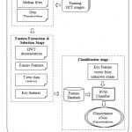 |
Figure 1: Proposed glaucoma diagnostic model using DWT |
From the segmented foreground region, the retinal region is automatically cropped for further processing. Also it is necessary that the resolution of input image to the proposed glaucoma diagnostic model should be similar.
Hence, the spatial resolution of the segmented region is adjusted to 64×128 pixels. In order to improve the image data for feature extraction it is necessary to denoise the image before segmentation. Hence, median filter of window size 7×7 is applied. Figure 2 shows the outputs at each stage of preprocessing of OCT images.
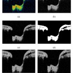 |
Figure 2: (a) Input OCT image (b) Gray scale image (c) Denoised image (d) Otsu thresholded image (e) Cropped image (f) Resolution adjusted image |
Feature Extraction and Selection Stage
Generally, lower dimensional representation of an image is named as feature vector and the process of extracting feature vector is called feature extraction. It plays a crucial role in determining and separating properties of glaucoma and non glaucoma patterns. Also, the accuracy of any classification system depends on the extracted discriminant features. In this study, features are extracted from OCT images in the frequency domain using wavelets.
To extract features in the wavelet domain, the pre-processed OCT images are initially subjected into DWT decomposition and the resultant wavelet coefficients are considered as features. As the images are 2-Dimenasional (2D) data, 2D-DWT is applied on the input image. In order to obtain 2D-DWT, 1D-DWT is applied along the rows one by one and then column wise. A pair of low pass and high pass filter is used for DWT decomposition [16]. The proposed system uses Haar wavelet for decomposition. Table 1 shows the low pass and high pass filter coefficients of Haar wavelet used in this study.
Table 1: Haar wavelet filter coefficients
| Low pass filter
coefficients |
High pass filter
coefficients |
| -0.01060 | -0.23038 |
| 0.03288 | 0.71485 |
| 0.03084 | -0.63088 |
| -0.18703 | -0.02798 |
| -0.02798 | 0.18703 |
| 0.63088 | 0.03084 |
| 0.71485 | -0.03288 |
DWT decomposition produces 4 sub-images at any level of decomposition as shown in figure 3 (a). For higher level of decomposition, the approximation sub-image is again considered for filtering as shown in figure 3 (b).
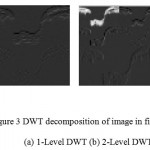 |
Figure 3: DWT decomposition of image in figure 2 (f) (a) 1-Level DWT (b) 2-Level DWT |
The dimension of DWT transformed image is exactly same as the input image size irrespective of the level of decomposition. Hence the dimension of the wavelet transformed image is 64×128 which means that there are 8192 wavelet coefficients available as features. As it is very high dimensional data, it will definitely affect the classification accuracy and also increases the computation time. To avoid these conditions, salient or key features are selected.
In this study t-test class separability criterion [17] is adopted for feature selection. The selected key feature set is used to classify the glaucomatous and non glaucomatous class of OCT images. It provides many benefits including improved classifier learning, improved predictive accuracy, reduced execution time and computational cost. The process of feature extraction and feature selection is performed for training OCT images and their corresponding features are stored for classifier training and testing.
Classification Stage
This is the final stage of the proposed glaucoma diagnostic model which helps ophthalmologists for early diagnosis and progression of glaucoma disease using OCT images. The classification accuracy of a system depend not only the selection of feature set but also the selection of optimal classifier. In this study, supervised learning approach based SVM classifier is adopted due to its superior generality and fast convergence in high dimensional data [18]. SVM classifier requires an open training session where only the input feature vectors of normal and glaucoma images are given along with their labels. In the training phase of SVM classification the relationship between the given features of normal and glaucoma is determined and optimized by means of hyperplane. It separates the given wavelet features optimally into two classes.
In order to diagnose the unknown OCT image for glaucoma, the top ranked key features are extracted by applying the “feature extraction and selection procedure” of training images. Then the extracted key features are fed to the trained SVM classifier wherein the unknown OCT image is labelled into glaucomatous or non glaucomatous based on feature space learning. In this study five various kernel functions such as linear, quadratic, polynomial, Radial Basis Function (RBF) and Multilayer Perceptron (MLP) are employed to analyze the performance of the proposed glaucoma diagnostic model.
Results and Discussions
This section discusses the performance of the proposed glaucoma diagnostic system based on DWT and SVM classifier. The assessment is carried on using 200 OCT images. Among them, 100 abnormal OCT images are obtained from glaucoma patients and the remaining images from healthy subjects. The images in the database are RGB images of size 689×329 pixels in the jpeg format, which is converted into gray scale for this study. Table 2 shows the accuracy of the proposed system for glaucoma diagnosis using cross validation process. R10 indicates that 10% of top ranked wavelet coefficients are used for classification process. The dataset used for evaluation is divided into 1/3rd of samples 10 times randomly. In each experiment, one sample is used for training the SVM classifier and the remaining samples used to test the proposed glaucoma diagnosis model. The statistics shown in the table 2 is the mean of 10 experiments.
It is evident from the above table 2 that the proposed system can able to classify the normal and glaucoma affected images with an accuracy of 90.75%, 80.12%, 83.82%, 80.26% and 76.32% for linear, quadratic, polynomial, RBF and MLP kernel respectively. It is also observed from the results that the linear kernel produces higher accuracy than other kernels used in this study. This is due to that linear kernel is the best choice if the number of features used for classification is higher. Also, the non linear mapping of high dimensional features is not able to improve the performance.
Table 2: Performance of the proposed glaucoma diagnostic system using SVM classifier
| SVM
Kernel |
DWT
Level |
Classification Accuracy (%) | ||||
| R10 | R20 | R30 | R40 | R50 | ||
| Linear | 1 | 67.32 | 78.92 | 79.16 | 76.40 | 70.86 |
| 2 | 77.97 | 82.31 | 83.36 | 80.57 | 78.50 | |
| 3 | 81.84 | 78.93 | 80.78 | 79.52 | 77.63 | |
| 4 | 79.47 | 81.33 | 81.94 | 79.76 | 78.04 | |
| 5 | 79.37 | 83.58 | 80.63 | 80.37 | 78.01 | |
| 6 | 79.87 | 84.61 | 84.43 | 90.75 | 81.08 | |
| Quadratic | 1 | 64.89 | 66.44 | 69.73 | 68.30 | 70.86 |
| 2 | 75.43 | 69.06 | 72.14 | 72.87 | 73.82 | |
| 3 | 73.78 | 67.58 | 72.35 | 73.78 | 72.23 | |
| 4 | 76.17 | 69.78 | 72.03 | 74.43 | 74.27 | |
| 5 | 76.02 | 77.66 | 76.63 | 78.67 | 80.12 | |
| 6 | 70.29 | 71.51 | 76.13 | 78.54 | 79.01 | |
| Polynomial | 1 | 62.68 | 70.58 | 73.96 | 77 | 78.47 |
| 2 | 74.54 | 74.67 | 73.44 | 77.80 | 79.04 | |
| 3 | 69.16 | 75.15 | 73.75 | 74.35 | 77.05 | |
| 4 | 70.88 | 74.29 | 76.06 | 79.03 | 79.62 | |
| 5 | 73.59 | 77.87 | 82.32 | 83.82 | 80.94 | |
| 6 | 70.10 | 72.04 | 73.87 | 75.78 | 75.85 | |
| RBF | 1 | 68.17 | 71.38 | 60.57 | 51.75 | 50 |
| 2 | 75.53 | 72.23 | 59.25 | 55.59 | 50.44 | |
| 3 | 78.32 | 68.11 | 60 | 51.47 | 50.88 | |
| 4 | 78.44 | 72.87 | 62.87 | 57.55 | 50.60 | |
| 5 | 80.26 | 72.78 | 59.06 | 50.73 | 49.67 | |
| 6 | 75.54 | 68.81 | 57 | 50.43 | 50 | |
| MLP | 1 | 59.38 | 67.43 | 73.44 | 74.60 | 71.37 |
| 2 | 68.90 | 69.49 | 72.18 | 73.07 | 71.67 | |
| 3 | 70.32 | 70.84 | 68.78 | 72.90 | 71.02 | |
| 4 | 67.33 | 73.43 | 73.05 | 69.13 | 71.48 | |
| 5 | 70.92 | 72.13 | 73.53 | 76.32 | 73.28 | |
| 6 | 69.06 | 74.53 | 74.40 | 75.68 | 75.45 | |
The performance of the proposed system increases while increasing the percentage of key features and level of DWT decomposition used for classification. The higher level of decomposition and more than 50% of top ranked features affects the performance due to the fact that the DWT produces redundant data at higher decomposition.
The performance of the proposed system is further analyzed by using confusion matrix and Receiver Operating Characteristics (ROC) curve. Figure 4 shows the confusion matrix and ROC curve corresponding to the features extracted at 6th level decomposition with selected R40 features for classification.
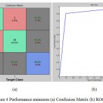 |
Figure 4: Performance measures (a) Confusion Matrix (b) ROC curve |
From the ROC curve, it is observed that the area under the curve is 0.908 that shows the capability of the classifier performance for classifying fundus images into either normal or glaucoma. It is clearly observed from the confusion matrix of the proposed system only misclassifies 3 images as normal instead of glaucomatous and 3 images as glaucomatous instead of normal among 65 testing images (33 images are glaucomatous and 32 images are normal). In order to analyze the extracted wavelet features, box plot analysis is used. Figure 5 shows the box plot for first top 2 ranked features extracted at 6th DWT decomposition level.
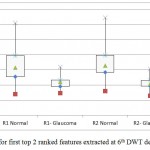 |
Figure 5: Box plot for first top 2 ranked features extracted at 6th DWT decomposition level. |
The performance of the proposed system is compared with the state-of-art dimension reduction technique i.e., PCA. Figure 6 shows the performance of the proposed system for five difference kernels in SVM classifier.
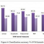 |
Figure 6: Classification accuracy Vs SVM kernels |
It is observed from the figure 6 that PCA based approach achieves maximum classification accuracy of only 75.80%. The reason is that PCA approach maximizes the within-class scatter which may affect the classification rate of the glaucoma diagnosis system. Among the five various kernel functions, quadratic approach achieves maximum classification accuracy than other kernel function while using PCA based features.
Conclusion
In this study, an early glaucoma detection system is proposed in wavelet domain using OCT images to prevent the onset of blindness. At first, OCT images undergo pre-processing stage where de-noising and cropping of retinal region is performed. Then, wavelet coefficients are obtained by DWT decomposition of pre-processed OCT image and key features are selected using statistical significance test. Finally, SVM classifier is employed for glaucomatous and healthy OCT image classification. It is observed from the experimental results that the proposed system achieves satisfactory performance over PCA and achieves maximum classification accuracy of 90.75%. Also the proposed approach yields sensitivity of 91.79%, and specificity of 89.71%.
References
- Schuman, J. S., Hee, M. R., Arya, A. V., Pedut-Kloizman, T., Puliafito, C. A., Fujimoto, J. G., & Swanson, E. A., Optical coherence tomography: a new tool for glaucoma diagnosis. Current opinion in ophthalmology., 1995; 6 (2): 89-95.
- Rajan, A & Ramesh, G. P, Glaucomatous Image Classification Based on PCA using Optical Coherence Tomography Images. International Journal of Applied Engineering Research., 2015; 10(17): 1-5.
- Rajan, A., Ramesh, G. P., & Yuvaraj, Glaucomatous image Classification using Wavelet Transform. IEEE International Conference on Advanced Communication Control and Computing Technologies., 2014; 1398-1402: DOI: 10.1109/ICACCCT.2014.7019330.
- Boyer, K. L., Herzog, A., & Roberts, C., Automatic recovery of the optic nerve head geometry in optical coherence tomography. IEEE Transaction on Medical Imaging., 2006; 25(5): 553-570. DOI: 1109/TMI.2006.871417.
- Tian, J., Marziliano, P., Baskaran, M., Wong, H. T., & Aung, T., Automatic anterior chamber angle assessment for HD-OCT images. IEEE Transaction on Biomedical Engineering,. 2011; 58 (11): 3242-3249. DOI: 1109/TBME.2011.2166397.
- Ojima, T., Tanabe, T., Hangai, M., Yu, S., Morishita, S., & Yoshimura, N, Measurement of retinal nerve fiber layer thickness and macular volume for glaucoma detection using optical coherence tomography. Japanese Journal of Ophthalmology., 2007; 51(3): 197-203.
- Chen, H. Y., & Huang, M. L., Discrimination between normal and glaucomatous eyes using Stratus optical coherence tomography in Taiwan Chinese subjects. Graefe’s Arch for Clinical and Experimental Ophthalmology., 2005; 243 (9): 894-902.
- Cvenkel, B., & Kontestabile, A. S., Correlation between nerve fibre layer thickness measured with spectral domain OCT and visual field in patients with different stages of glaucoma. Graefe’s Arch for Clinical and Experimental Ophthalmology., 2011; 249(4): 575-584.DOI: 1007/s00417-010-1538-z.
- Burgansky-Eliash, Z., Wollstein, G., Chu, T., Ramsey, J. D., Glymour, C., Noecker, R. J. & Schuman, J. S., Optical coherence tomography machine learning classifiers for glaucoma detection: a preliminary study. Investigative Ophthalmology & Visual Science.,2005; 46 (11): 4147-4152. DOI: 1167/iovs.05-0366.
- Koprowski, R., Rzendkowski, M., & Wróbel, Z., Automatic method of analysis of OCT images in assessing the severity degree of glaucoma and the visual field loss. Biomed engineering online, 2014; 13 (1): 1-18. DOI: 1186/1475-925X-13-16.
- Ganeshbabu, T. R., Devi, S. S., & Venkatesh, R., Automatic Detection of Glaucoma Using Optical Coherence Tomography Image. Journal of Applied Sciences., 2012; 12: 2128-2138.DOI: 10.3923/jas.2012.2128.2138.
- Huang, M. L., Chen, H. Y., & Hung, T., Analysis of glaucoma diagnosis with automated classifiers using stratus optical coherence tomography. Optical and quantum electronics., 2005; 37(13-15): 1239-1249.DOI: 1007/s11082-005-4195-4.
- Huang, M. L., Chen, H. Y., & Huang, J. J., Glaucoma detection using adaptive neuro-fuzzy inference system. Expert System with Application, 2007; 32(2): 458-468.
- Zhu, H., Crabb, D. P., Schlottmann, P. G., Wollstein, G., & Garway-Heath, D. F., Aligning scan acquisition circles in optical coherence tomography images of the retinal nerve fibre layer. IEEE Transaction on Medical Imaging, 2011; 30(6): 1228-1238.DOI: 1109/TMI.2011.2109962
- Otsu, N., A Threshold Selection Method from Gray-Level Histograms, IEEE Transactions on Systems, Man, and Cybernetics. 1979; 9(1): 62-66. DOI: 1109/TSMC.1979.4310076.
- G.Mallat, A theory for multi resolution signal Decomposition: The wavelet representation, IEEE transactions on pattern analysis and machine intelligence., 1989; 11(7): 674-693.DOI: 10.1109/34.192463.
- Wei Zhu, Xuena Wang, Yeming Ma, Manlong Rao, James Glimm, and John S. Kovach, Detection of cancer-specific markers amid massive mass spectral data, Proceedings of the National Academy of Sciences, 2003; 100(25): 14666-14671.
- Vapnik, V. N., Statistical learning theory, Wiley New York, 1998.
(Visited 486 times, 1 visits today)

This work is licensed under a Creative Commons Attribution 4.0 International License.


